Using the Taiwan AirBox Data in Example 5.5, compare the clustering results obtained using the ACF and

Question:

Using the Taiwan AirBox Data in Example 5.5, compare the clustering results obtained using the ACF and using the coefficients of an AR fitting to the series.

Data From Example 5.5:

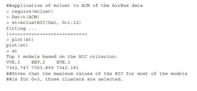
We used the mclust package for model-based clustering of the Taiwan AirBox data.
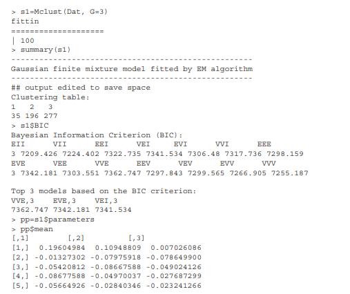
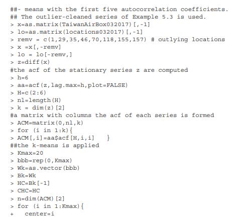
The series are summarized by the first five autocorrelation coefficients. The R commands used are given below. We do not repeat the computation of the ACM matrix as it is the same as that of Example 5.4. The main command is mclustBIC, that provides a summary of the values of the BIC as approximations to the posterior probabilities of the model under different scenarios, given by the structure of the covariance matrices in the mixture of normals. Once the number of clusters is chosen, the command Mclust gives the estimation result of the mixture model.

R commands for model-based clustering with package mclust:

image text in transcribed

Example 5.4:

We apply \(k\)-means to the TaiwanAirBox data. We use the set of 508 time series after removing eight series with six of them associated with outlying locations and two series with only a few non-zero data points. See Example 5.3. The R command kmeans is used, which is in the stats package. Three types of variables of different dimensions are used. The first type consists of the first 5 lags of ACF of each series so \(p=5\); the second type is the average value of the series in each of the 31 days in the sample so that \(p=31\); and the third type uses every observation of the time series as a variable so that we have \(p=T=743\). The number of clusters is selected using the Calinski and Harabasz criterion \((\mathrm{CHC})\), that is computed below. A maximum of 20 clusters are allowed and, for each number of groups, \(k\)-means is applied with 10 random starting values and the value of the criterion is saved in the vector \(\mathrm{CHC}\).

R commands for k-means:

image text in transcribed

Example 5.3:

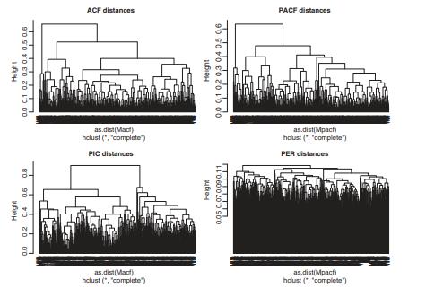
Consider, again, the Taiwan AirBox and the New England electricity price data in the files TaiwanAirBox032017.csv and Pelectricity1344.csv, respectively, but use the first differenced series, that is, \(\boldsymbol{z}_t=abla \boldsymbol{x}_t\), where \(\boldsymbol{x}_t\) is the observed time series. As before, we removed Series 29 and 70 from the AirBox data set. Figure 5.12 shows the dendrograms of the hierarchical clustering results for the AirBox data based on four distance measures, which are the first 5 lags of ACF and PACF, the PIC distance with AR order selected automatically, and the PER. From the plots, the PACF and PIC distances seem to provide similar clustering results. This is not surprising as PACF is closely related to the AR coefficients. The PER distance, on the other hand, seems to provide slightly different results. We then apply the silhouette and gap statistics with the ACF distance to the data set. The silhouette statistic suggests two clusters whereas the gap statistic indicates four clusters. Furthermore, based on the ACF distance, if we select three clusters, then the cluster sizes are 390,107 , and 17 , respectively. The \(\mathrm{R}\) commands and packages used and some outputs are given below, where the command hclust, for hierarchical clustering, is part of the R package stats.

Figure 5.12: