

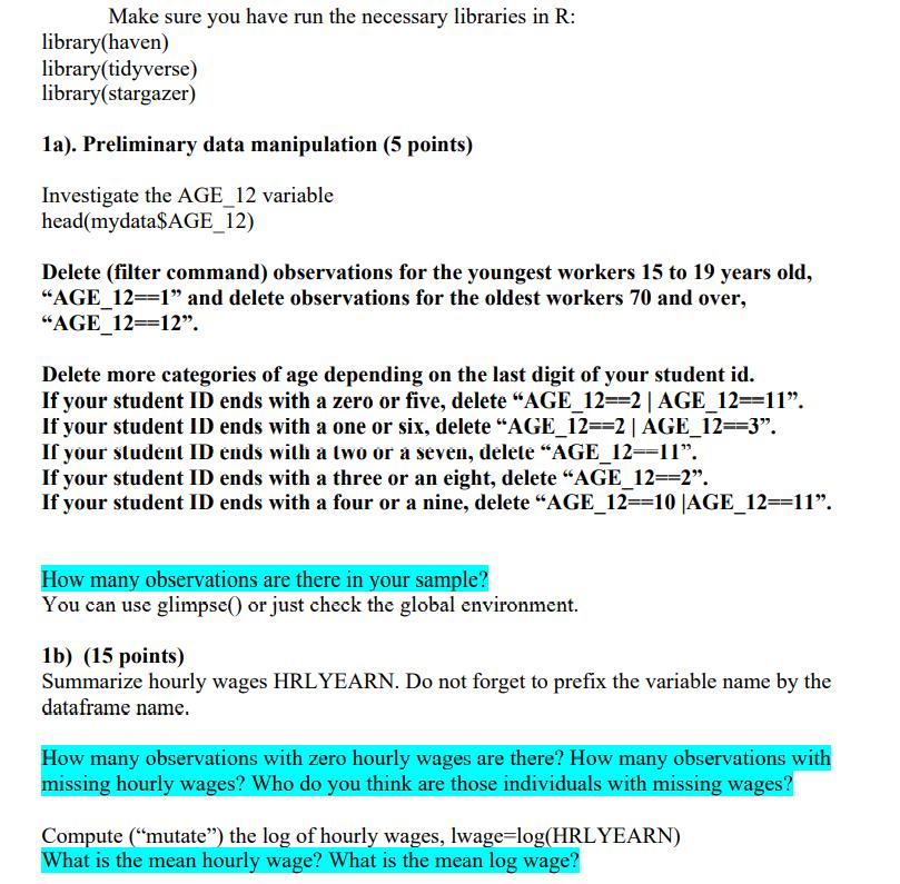
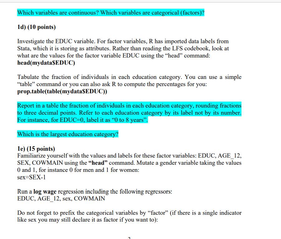
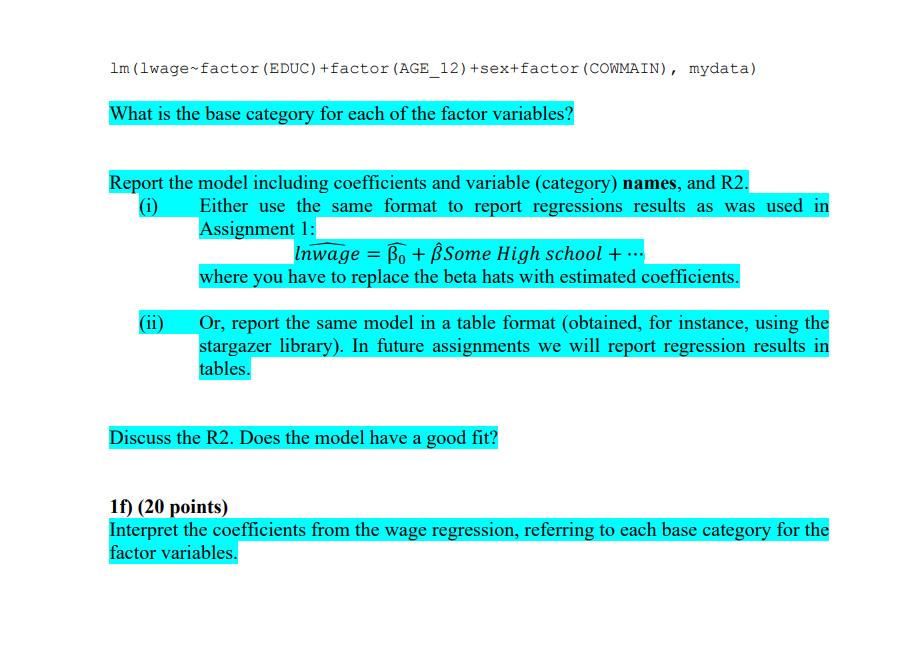
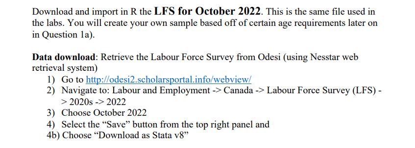
Make sure you have run the necessary libraries in R: library(haven) library(tidyverse) library(stargazer) 1a). Preliminary data...
Fantastic news! We've Found the answer you've been seeking!
Question:

Transcribed Image Text:
Make sure you have run the necessary libraries in R: library(haven) library(tidyverse) library(stargazer) 1a). Preliminary data manipulation (5 points) Investigate the AGE_12 variable head(mydata$AGE_12) Delete (filter command) observations for the youngest workers 15 to 19 years old, "AGE_12=1" and delete observations for the oldest workers 70 and over, "AGE_12=12". Delete more categories of age depending on the last digit of your student id. If your student ID ends with a zero or five, delete "AGE_12=-2 |AGE_12==11". If your student ID ends with a one or six, delete "AGE_12==2 | AGE_12==3. If your student ID ends with a two or a seven, delete "AGE_12--11". If your student ID ends with a three or an eight, delete "AGE_12==2". If your student ID ends with a four or a nine, delete "AGE_12=-10 |AGE_12=11". How many observations are there in your sample? You can use glimpse() or just check the global environment. 1b) (15 points) Summarize hourly wages HRLYEARN. Do not forget to prefix the variable name by the dataframe name. How many observations with zero hourly wages are there? How many observations with missing hourly wages? Who do you think are those individuals with missing wages? Compute ("mutate") the log of hourly wages, lwage=log(HRLYEARN) What is the mean hourly wage? What is the mean log wage? Note: the simplest way to make a histogram (using the ggplot visualisation from the tidiverse library): ggplot (mydata, aes (x-HRLYEARN)) + geom_histogram () ggplot (mydata, aes (x=lwage)) + geom_histogram () These plots are a basic and you can improve on the visualisation if you are feeling ambitious by adding parameters to the ggplot commands (In the answer key I will leave it as in the basic example from above). Here is one possible source for inspiration (there are many): http://www.sthda.com/english/wiki/ggplot2-histogram-plot-quick-start-guide-r- software-and-data-visualization 2 From here on use the dataframe with non-missing lwage. filter (!is.na (lwage)) It is not a bad idea to give the dataframe a new name at this point. 1c) (5 points) Consider the following variables: HRLYEARN AGE_12 EDUC SEX COWMAIN UNION Investigate each variable either from the drop-down arrow in the global environment or using the "head" or "glimpse" commands, e.g. glimpse(mydata$HRLYEARN) Which variables are continuous? Which variables are categorical (factors)? 1d) (10 points) Investigate the EDUC variable. For factor variables, R has imported data labels from Stata, which it is storing as attributes. Rather than reading the LFS codebook, look at what are the values for the factor variable EDUC using the "head" command: head(mydata$EDUC) Tabulate the fraction of individuals in each education category. You can use a simple "table" command or you can also ask R to compute the percentages for you: prop.table(table(mydata$EDUC)) Report in a table the fraction of individuals in each education category, rounding fractions to three decimal points. Refer to each education category by its label not by its number. For instance, for EDUC=0, label it as "0 to 8 years". Which is the largest education category? 1e) (15 points) Familiarize yourself with the values and labels for these factor variables: EDUC, AGE_12, SEX, COWMAIN using the "head" command. Mutate a gender variable taking the values O and 1, for instance 0 for men and 1 for women: sex-SEX-1 Run a log wage regression including the following regressors: EDUC, AGE_12, sex, COWMAIN Do not forget to prefix the categorical variables by "factor" (if there is a single indicator like sex you may still declare it as factor if you want to): 1m (1wage factor (EDUC) +factor (AGE_12) +sex+factor (COWMAIN), mydata) What is the base category for each of the factor variables? Report the model including coefficients and variable (category) names, and R2. Either use the same format to report regressions results as was used in Assignment 1: (i) (ii) Inwage=Bo+ Some High school+... where you have to replace the beta hats with estimated coefficients. Or, report the same model in a table format (obtained, for instance, using the stargazer library). In future assignments we will report regression results in tables. Discuss the R2. Does the model have a good fit? 1f) (20 points) Interpret the coefficients from the wage regression, referring to each base category for the factor variables. Download and import in R the LFS for October 2022. This is the same file used in the labs. You will create your own sample based off of certain age requirements later on in Question la). Data download: Retrieve the Labour Force Survey from Odesi (using Nesstar web retrieval system) 1) Go to http://odesi2.scholarsportal.info/webview/ 2) Navigate to: Labour and Employment -> Canada -> Labour Force Survey (LFS) - > 2020s -> 2022 3) Choose October 2022 4) Select the "Save" button from the top right panel and 4b) Choose "Download as Stata v8" Make sure you have run the necessary libraries in R: library(haven) library(tidyverse) library(stargazer) 1a). Preliminary data manipulation (5 points) Investigate the AGE_12 variable head(mydata$AGE_12) Delete (filter command) observations for the youngest workers 15 to 19 years old, "AGE_12=1" and delete observations for the oldest workers 70 and over, "AGE_12=12". Delete more categories of age depending on the last digit of your student id. If your student ID ends with a zero or five, delete "AGE_12=-2 |AGE_12==11". If your student ID ends with a one or six, delete "AGE_12==2 | AGE_12==3. If your student ID ends with a two or a seven, delete "AGE_12--11". If your student ID ends with a three or an eight, delete "AGE_12==2". If your student ID ends with a four or a nine, delete "AGE_12=-10 |AGE_12=11". How many observations are there in your sample? You can use glimpse() or just check the global environment. 1b) (15 points) Summarize hourly wages HRLYEARN. Do not forget to prefix the variable name by the dataframe name. How many observations with zero hourly wages are there? How many observations with missing hourly wages? Who do you think are those individuals with missing wages? Compute ("mutate") the log of hourly wages, lwage=log(HRLYEARN) What is the mean hourly wage? What is the mean log wage? Note: the simplest way to make a histogram (using the ggplot visualisation from the tidiverse library): ggplot (mydata, aes (x-HRLYEARN)) + geom_histogram () ggplot (mydata, aes (x=lwage)) + geom_histogram () These plots are a basic and you can improve on the visualisation if you are feeling ambitious by adding parameters to the ggplot commands (In the answer key I will leave it as in the basic example from above). Here is one possible source for inspiration (there are many): http://www.sthda.com/english/wiki/ggplot2-histogram-plot-quick-start-guide-r- software-and-data-visualization 2 From here on use the dataframe with non-missing lwage. filter (!is.na (lwage)) It is not a bad idea to give the dataframe a new name at this point. 1c) (5 points) Consider the following variables: HRLYEARN AGE_12 EDUC SEX COWMAIN UNION Investigate each variable either from the drop-down arrow in the global environment or using the "head" or "glimpse" commands, e.g. glimpse(mydata$HRLYEARN) Which variables are continuous? Which variables are categorical (factors)? 1d) (10 points) Investigate the EDUC variable. For factor variables, R has imported data labels from Stata, which it is storing as attributes. Rather than reading the LFS codebook, look at what are the values for the factor variable EDUC using the "head" command: head(mydata$EDUC) Tabulate the fraction of individuals in each education category. You can use a simple "table" command or you can also ask R to compute the percentages for you: prop.table(table(mydata$EDUC)) Report in a table the fraction of individuals in each education category, rounding fractions to three decimal points. Refer to each education category by its label not by its number. For instance, for EDUC=0, label it as "0 to 8 years". Which is the largest education category? 1e) (15 points) Familiarize yourself with the values and labels for these factor variables: EDUC, AGE_12, SEX, COWMAIN using the "head" command. Mutate a gender variable taking the values O and 1, for instance 0 for men and 1 for women: sex-SEX-1 Run a log wage regression including the following regressors: EDUC, AGE_12, sex, COWMAIN Do not forget to prefix the categorical variables by "factor" (if there is a single indicator like sex you may still declare it as factor if you want to): 1m (1wage factor (EDUC) +factor (AGE_12) +sex+factor (COWMAIN), mydata) What is the base category for each of the factor variables? Report the model including coefficients and variable (category) names, and R2. Either use the same format to report regressions results as was used in Assignment 1: (i) (ii) Inwage=Bo+ Some High school+... where you have to replace the beta hats with estimated coefficients. Or, report the same model in a table format (obtained, for instance, using the stargazer library). In future assignments we will report regression results in tables. Discuss the R2. Does the model have a good fit? 1f) (20 points) Interpret the coefficients from the wage regression, referring to each base category for the factor variables. Download and import in R the LFS for October 2022. This is the same file used in the labs. You will create your own sample based off of certain age requirements later on in Question la). Data download: Retrieve the Labour Force Survey from Odesi (using Nesstar web retrieval system) 1) Go to http://odesi2.scholarsportal.info/webview/ 2) Navigate to: Labour and Employment -> Canada -> Labour Force Survey (LFS) - > 2020s -> 2022 3) Choose October 2022 4) Select the "Save" button from the top right panel and 4b) Choose "Download as Stata v8"
Expert Answer:

Related Book For 

Measurement Theory In Action
ISBN: 9780367192181
3rd Edition
Authors: Kenneth S Shultz, David Whitney, Michael J Zickar
Posted Date:
Students also viewed these economics questions
-
Discuss how lean production could work in the service sector.What can you imagine it would take to implement?How might you measure the effectiveness of your suggestions?Provide an example. Your...
-
Planning is one of the most important management functions in any business. A front office managers first step in planning should involve determine the departments goals. Planning also includes...
-
Q1. You have identified a market opportunity for home media players that would cater for older members of the population. Many older people have difficulty in understanding the operating principles...
-
Which one the below does not define "Work role boundaries" of a care worker limits that allow a patient and staff to connect safely in a therapeutic relationship based on patients' needs rules of...
-
Potassium tert-butoxide reacts with halobenzenes on heating in dimethyl sulfoxide to give tert-butyl phenyl ether. (a) o-Fluorotoluene yields tert-butyl o-methylphenyl ether almost exclusively under...
-
Let \(f(\theta)\) be the \(2 \pi\)-periodic function determined by the formula \[f(\theta)=|\sin \theta|, \quad \text { for }-\pi \leq \theta \leq \pi\] Show that the Fourier series for \(f\) is...
-
If \(80 \%\) of the total is 60 , how much is in the total?
-
Projects A and B, of equal risk, are alternatives for expanding Rosa Company's capacity. The firm's cost of capital is 13%. The cash flows for each project are shown in the following table. a....
-
Exercise 22-14 (LO. 6)Dion, an S shareholder, owned 20% of MeadowBrook's stock for 292days and 25% for the remaining 73 days in the year. Using therequired per-day allocation method, compute Dion's 2...
-
You have correctly calculated the following ratios for Blue Royals Ltd. ("BLUR"): Quick ratio: 1.5 to 1 6 times Inventory turnover: Debt to equity: Profit margin: 2 to 1 (debt total liabilities) 30%...
-
Suppose during a TLC experiment the distance between the origin and one of the analytes was 4.5cm. What would be the retention factor if the distance between the origin and the solvent front was...
-
A particle is constrained to travel along the path as shown here. Let's say x = (5t4) m. Here t is in the units of seconds. Given y (4x) m. = Find the magnitudes of particle's velocity and...
-
A car takes a trip consisting of two displacements. The first displacement is 25 km [N], and the total displacement is 62 km [N 38 W]. Determine the second displacement. Find the direction as well.
-
You are a trader for GreekLetters Ltd. You have sold 100,000 put options on a stock at strike $24.5 and also short 50,000 of the stock. The options expire in 9 months. The stock is currently trading...
-
23. A thermal power has a net power 10 MW. The back work ratio of the plant is 0.005. Calculate the compressor work. A. 52.75 KW B. 56.50 KW C. 50.25 KW D. 42.55 KW
-
South Korean entertainment is (K-pop, K-drama etc.) is helping to increase the North American demand for Korean goods more broadly. 1. Consider the following questions: Imagine that one month ago...
-
Which property determines whether a control is available to the user during run time? a. Available b. Enabled c. Unavailable d. Disabled
-
Yale Corporation issued to Zap Corporation \(\$ 60,000,8 \%\) (cash interest payable semiannually on June 30 and December 31) 10 -year bonds dated and sold on January 1, 2020. Assume that the company...
-
Yale Corporation issued to Zap Corporation \(\$ 60,000,8 \%\) (cash interest payable semiannually on July 1 and January 1) 10 -year bonds dated and sold on January 1,2020 . If the bonds were sold at...
-
Lacey Corp. issued a three-year, \(\$ 5,000\) note with an \(8 \%\) stated rate to Hayley Co. on January 1, 2020, and received cash of \(\$ 5,000\). The note requires semiannual interest payments on...

Study smarter with the SolutionInn App