

10 6. 4. 5. 7. PROJECT STEPS Carla Arranga is a senior account manager at Ensight...
Fantastic news! We've Found the answer you've been seeking!
Question:
Transcribed Image Text:
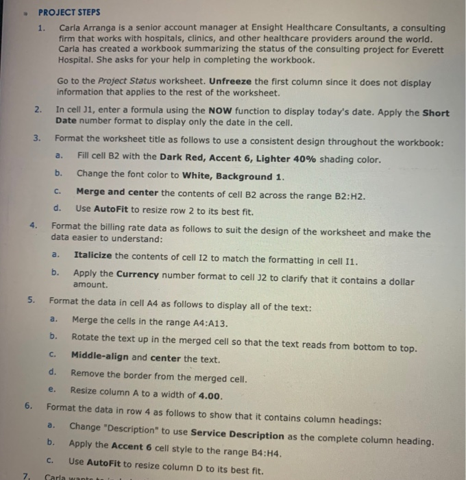
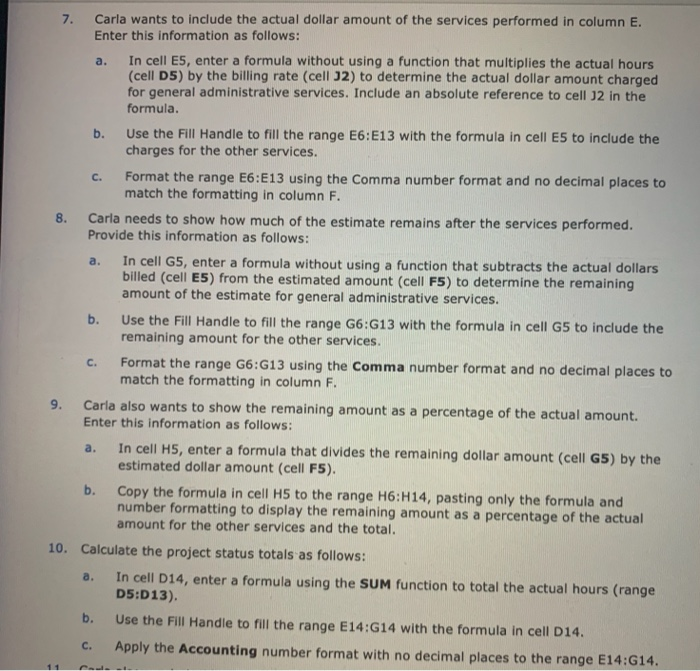
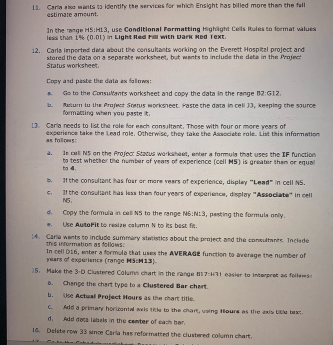
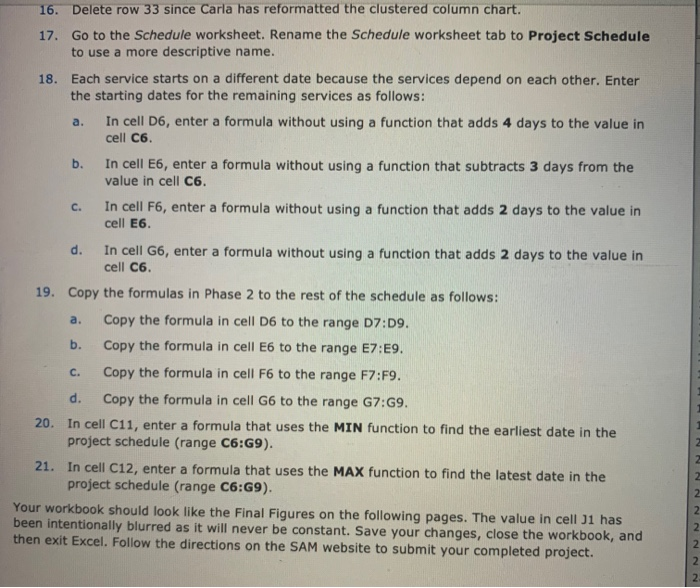
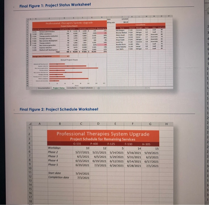
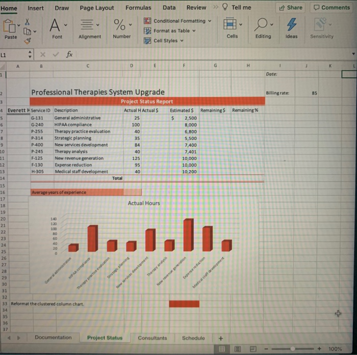
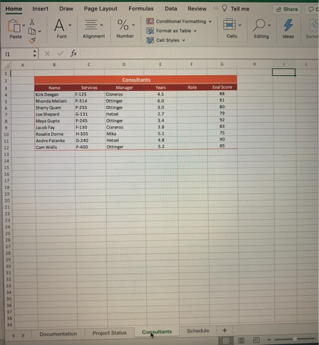
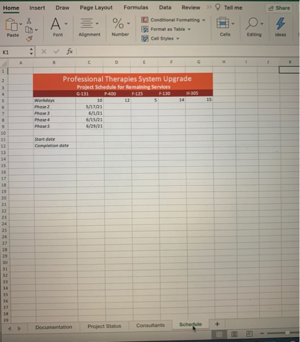
10 6. 4. 5. 7. PROJECT STEPS Carla Arranga is a senior account manager at Ensight Healthcare Consultants, a consulting firm that works with hospitals, clinics, and other healthcare providers around the world. Carla has created a workbook summarizing the status of the consulting project for Everett Hospital. She asks for your help in completing the workbook. 1. 2. In cell J1, enter a formula using the NOW function to display today's date. Apply the Short Date number format to display only the date in the cell. 3. Format the worksheet title as follows to use a consistent design throughout the workbook: Fill cell B2 with the Dark Red, Accent 6, Lighter 40% shading color. Change the font color to White, Background 1. Merge and center the contents of cell B2 across the range B2:H2. Use AutoFit to resize row 2 to its best fit. a. b. C. d. Format the billing rate data as follows to suit the design of the worksheet and make the data easier to understand: Go to the Project Status worksheet. Unfreeze the first column since it does not display information that applies to the rest of the worksheet. Italicize the contents of cell 12 to match the formatting in cell 11. Apply the Currency number format to cell J2 to clarify that it contains a dollar amount. Format the data in cell A4 as follows to display all of the text: Merge the cells in the range A4:A13. Rotate the text up in the merged cell so that the text reads from bottom to top. Middle-align and center the text. a. b. a. b. C. d. Remove the border from the merged cell. Resize column A to a width of 4.00. Format the data in row 4 as follows to show that it contains column headings: Change "Description" to use Service Description as the complete column heading. Apply the Accent 6 cell style to the range B4:H4. Use AutoFit to resize column D to its best fit. e. a. b. C. Carla wants t 7. 8. 9. 11 Carla wants to include the actual dollar amount of the services performed in column E. Enter this information as follows: a. b. C. a. b. Carla needs to show how much of the estimate remains after the services performed. Provide this information as follows: C. b. In cell E5, enter a formula without using a function that multiplies the actual hours. (cell D5) by the billing rate (cell 32) to determine the actual dollar amount charged for general administrative services. Include an absolute reference to cell 32 in the formula. Use the Fill Handle to fill the range E6: E13 with the formula in cell E5 to include the charges for the other services. C. Format the range E6:E13 using the Comma number format and no decimal places to match the formatting in column F. a. Carla also wants to show the remaining amount as a percentage of the actual amount. Enter this information as follows: b. In cell G5, enter a formula without using a function that subtracts the actual dollars billed (cell E5) from the estimated amount (cell F5) to determine the remaining amount of the estimate for general administrative services. a. In cell H5, enter a formula that divides the remaining dollar amount (cell G5) by the estimated dollar amount (cell F5). Use the Fill Handle to fill the range G6:G13 with the formula in cell G5 to include the remaining amount for the other services. Format the range G6:G13 using the Comma number format and no decimal places to match the formatting in column F. 10. Calculate the project status totals as follows: In cell D14, enter a formula using the SUM function to total the actual hours (range D5:D13). Use the Fill Handle to fill the range E14:G14 with the formula in cell D14. Apply the Accounting number format with no decimal places to the range E14:G14. Carlo - Copy the formula in cell H5 to the range H6:H14, pasting only the formula and number formatting to display the remaining amount as a percentage of the actual amount for the other services and the total. 11. Carla also wants to identify the services for which Ensight has billed more than the full estimate amount. In the range H5:H13, use Conditional Formatting Highlight Cells Rules to format values less than 1% (0.01) in Light Red Fill with Dark Red Text. 12. Carla imported data about the consultants working on the Everett Hospital project and stored the data on a separate worksheet, but wants to include the data in the Project Status worksheet. Copy and paste the data as follows: a. Go to the Consultants worksheet and copy the data in the range B2:G12. b. Return to the Project Status worksheet. Paste the data in cell 33, keeping the source formatting when you paste it. 13. Carla needs to list the role for each consultant. Those with four or more years of experience take the Lead role. Otherwise, they take the Associate role. List this information as follows: a. 17 b. C. d. e. 14. Carla wants to include summary statistics about the project and the consultants. Include this information as follows: In cell N5 on the Project Status worksheet, enter a formula that uses the IF function to test whether the number of years of experience (cell M5) is greater than or equal to 4. In cell D16, enter a formula that uses the AVERAGE function to average the number of years of experience (range M5:M13). 15. Make the 3-D Clustered Column chart in the range B17:H31 easier to interpret as follows: b. If the consultant has four or more years of experience, display "Lead" in cell N5. If the consultant has less than four years of experience, display "Associate" in cell N5. Change the chart type to a Clustered Bar chart. Use Actual Project Hours as the chart title. Add a primary horizontal axis title to the chart, using Hours as the axis title text. Add data labels in the center of each bar. 16. Delete row 33 since Carla has reformatted the clustered column chart. Besame M C. Copy the formula in cell N5 to the range N6:N13, pasting the formula only. Use AutoFit to resize column N to its best fit. d. 16. Delete row 33 since Carla has reformatted the clustered column chart. 17. Go to the Schedule worksheet. Rename the Schedule worksheet tab to Project Schedule to use a more descriptive name. 18. Each service starts on a different date because the services depend on each other. Enter the starting dates for the remaining services as follows: a. b. C. d. a. b. In cell D6, enter a formula without using a function that adds 4 days to the value in cell C6. C. In cell E6, enter a formula without using a function that subtracts 3 days from the value in cell C6. In cell F6, enter a formula without using a function that adds 2 days to the value in cell E6. 19. Copy the formulas in Phase to the rest of the schedule as follows: Copy the formula in cell D6 to the range D7:D9. Copy the formula in cell E6 to the range E7:E9. Copy the formula in cell F6 to the range F7:F9. Copy the formula in cell G6 to the range G7:G9. d. 20. In cell C11, enter a formula that uses the MIN function to find the earliest date in the project schedule (range C6:G9). In cell G6, enter a formula without using a function that adds 2 days to the value in cell C6. 21. In cell C12, enter a formula that uses the MAX function to find the latest date in the project schedule (range C6:G9). Your workbook should look like the Final Figures on the following pages. The value in cell J1 has been intentionally blurred as it will never be constant. Save your changes, close the workbook, and then exit Excel. Follow the directions on the SAM website to submit your completed project. 2. Final Figure 1: Project Status Worksheet 2 3 4 5 6 A A 1 7 8 9 10 11 6.340 PM PAN 12 13 14 POR 15 16 17 18 1.300 Professional Therapies System Upgrade Project Report at ping Total Final Figure 2: Project Schedule Worksheet A AMD 1,400 2419 7140 1400 W 10,425 ROS 1,400 504 49,040 . e 40 n 14 A B 125 Actual Project Houn Workdays Phase 2 Phase 3 Phase 4 Phase 5 Documentation Project Status Consultants Project Schedule K Sumbing Bemary's 2,500 $ A000 LACK 1,00 1400 1401 4,301 10000 ( 10.000 LAUS AND 10,300 ONS HE Start date Completion date с ( KAD 2425 10 D 5/14/2021 7/3/2021 Dete ang AN SON AN 4V MAN AN 196 47% 2PM 12 R VER Dengan Wonde Malled Sherry Quan ce Food Maya Ga cay 545.00 E Park Can Wells Sva F-LIS Pa P-255 G-I P-345 Consultant Professional Therapies System Upgrade Project Schedule for Remaining Services G-131 P-400 F-125 F-130 5 Penager Tre Oninger Odingar PAM Onger Ostern H-301 Mia Metal 64 400 5.4 4.4 $3 1.8 Associate BE lead 71 90 W Bilde Associate Associate 14 15 5/17/2021 5/21/2021 5/14/2021 5/16/2021 5/19/2021 6/1/2021 6/5/2021 5/29/2021 5/31/2021 6/3/2021 6/15/2021 6/19/2021 6/12/2021 6/14/2021 6/17/2021 6/29/2021 7/3/2021 6/26/2021 6/28/2021 7/1/2021 H-305 Lead H 1 2 3 4 5 8 9 10 1 15 INNN22 3 Home L1 1 Paste 2 8 9 10 11 12 13 14 15 16 17 18 19 20 21 22 23 24 25 26 A Insert 35 36 37 X V 3 4 Everett H Service ID Description S 6 7 x B Draw Page Layout G-131 G-240 P-255 P-314 A = Font P-400 P-245 F-125 F-130 H-305 ✓ fx Alignment General administrative HIPAA compliance Therapy practice evaluation Strategic planning New services development Therapy analysis New revenue generation Professional Therapies System Upgrade Project Status Report Actual H Actual S$ 25 100 40 35 84 40 Expense reduction Medical staff development 140 120 100 80 60 40 20 с Average years of experience D 27 28 29 30 31 32 33 Reformat the clustered column chart. 34 HIPAA compliance General administrative Documentation %* Number Therapy practice evaluation Formulas Total D Project Status 125 95 40 Conditional Formatting ✓ Format as Table Cell Styles E Strategic planning Actual Hours Data Review >> ......... New services development Therapy analysis F Estimated $ $ Consultants 2,500 8,000 6,800 5,500 7,400 7,401 10,000 10,000 10,200 New revenue generation Expense reduction G Schedule Tell me Cells Remaining $ Remaining % Medical staff development + H O. Editing E [U] Date: 1 Share 4 Ideas Billing rate: J Comments Sensitivity 85 100% Home 11 1 2 3 4 5 6 7 8 9 10 11 12 13 14 15 16 Paste 17 7 18 19 20 12 23 24 25 26 27 28 29 30 31 32 38 3 35 36 D 38 39 22 33 34 37 A Insert Draw Page Layout A- V Font x B ✓ fx Name Kirk Deegan Rhonda Meilani Sherry Quam Joe Shepard Maya Gupta Jacob Fay Rosalie Dorne Andre Patanka Cam Wells Alignment F-125 P-314 P-255 Services G-131 P-245 Documentation с F-130 H-305 G-240 P-400 %* Number D Consultants Manager Cisneros Ottinger Ottinger Hetzel Formulas Ottinger Cisneros Mika Hetzel Ottinger Project Status Data Review Conditional Formatting Format as Table Cell Styles E Years 4.5 6.0 3.0 2.7 3.4 3.8 5.1 4.8 5.2 Consultants F Role Schedule G Tell me Cells Eval Score 88 91 80 79 92 83 75 90 85 + V Editing H E1 Share 4 Ideas Sensit Home Insert K1 1 2 3 4 5 6 7 8 9 10 11 12 13 Paste 14 15 16 17 18 19 20 21 22 23 24 25 26 27 28 29 30 31 32 33 34 35 36 37 38 39 A Draw Page Layout A. Font x ✓ fx B Workdays Phase 2 Phase 3 Phase 4 Phase 5 Start date Completion date E Alignment Documentation C 10 5/17/21 6/1/21 6/15/21 6/29/21 Formulas %* Number Professional Therapies System Upgrade Project Schedule for Remaining Services G-131 P-400 F-125 F-130 Project Status E 12 Data Review >> Conditional Formatting Format as Table Cell Styles 5 Consultants 14 G H-305 Schedule 15 Tell me Cells H Editing I E1 1 Share Ideas K 10 6. 4. 5. 7. PROJECT STEPS Carla Arranga is a senior account manager at Ensight Healthcare Consultants, a consulting firm that works with hospitals, clinics, and other healthcare providers around the world. Carla has created a workbook summarizing the status of the consulting project for Everett Hospital. She asks for your help in completing the workbook. 1. 2. In cell J1, enter a formula using the NOW function to display today's date. Apply the Short Date number format to display only the date in the cell. 3. Format the worksheet title as follows to use a consistent design throughout the workbook: Fill cell B2 with the Dark Red, Accent 6, Lighter 40% shading color. Change the font color to White, Background 1. Merge and center the contents of cell B2 across the range B2:H2. Use AutoFit to resize row 2 to its best fit. a. b. C. d. Format the billing rate data as follows to suit the design of the worksheet and make the data easier to understand: Go to the Project Status worksheet. Unfreeze the first column since it does not display information that applies to the rest of the worksheet. Italicize the contents of cell 12 to match the formatting in cell 11. Apply the Currency number format to cell J2 to clarify that it contains a dollar amount. Format the data in cell A4 as follows to display all of the text: Merge the cells in the range A4:A13. Rotate the text up in the merged cell so that the text reads from bottom to top. Middle-align and center the text. a. b. a. b. C. d. Remove the border from the merged cell. Resize column A to a width of 4.00. Format the data in row 4 as follows to show that it contains column headings: Change "Description" to use Service Description as the complete column heading. Apply the Accent 6 cell style to the range B4:H4. Use AutoFit to resize column D to its best fit. e. a. b. C. Carla wants t 7. 8. 9. 11 Carla wants to include the actual dollar amount of the services performed in column E. Enter this information as follows: a. b. C. a. b. Carla needs to show how much of the estimate remains after the services performed. Provide this information as follows: C. b. In cell E5, enter a formula without using a function that multiplies the actual hours. (cell D5) by the billing rate (cell 32) to determine the actual dollar amount charged for general administrative services. Include an absolute reference to cell 32 in the formula. Use the Fill Handle to fill the range E6: E13 with the formula in cell E5 to include the charges for the other services. C. Format the range E6:E13 using the Comma number format and no decimal places to match the formatting in column F. a. Carla also wants to show the remaining amount as a percentage of the actual amount. Enter this information as follows: b. In cell G5, enter a formula without using a function that subtracts the actual dollars billed (cell E5) from the estimated amount (cell F5) to determine the remaining amount of the estimate for general administrative services. a. In cell H5, enter a formula that divides the remaining dollar amount (cell G5) by the estimated dollar amount (cell F5). Use the Fill Handle to fill the range G6:G13 with the formula in cell G5 to include the remaining amount for the other services. Format the range G6:G13 using the Comma number format and no decimal places to match the formatting in column F. 10. Calculate the project status totals as follows: In cell D14, enter a formula using the SUM function to total the actual hours (range D5:D13). Use the Fill Handle to fill the range E14:G14 with the formula in cell D14. Apply the Accounting number format with no decimal places to the range E14:G14. Carlo - Copy the formula in cell H5 to the range H6:H14, pasting only the formula and number formatting to display the remaining amount as a percentage of the actual amount for the other services and the total. 11. Carla also wants to identify the services for which Ensight has billed more than the full estimate amount. In the range H5:H13, use Conditional Formatting Highlight Cells Rules to format values less than 1% (0.01) in Light Red Fill with Dark Red Text. 12. Carla imported data about the consultants working on the Everett Hospital project and stored the data on a separate worksheet, but wants to include the data in the Project Status worksheet. Copy and paste the data as follows: a. Go to the Consultants worksheet and copy the data in the range B2:G12. b. Return to the Project Status worksheet. Paste the data in cell 33, keeping the source formatting when you paste it. 13. Carla needs to list the role for each consultant. Those with four or more years of experience take the Lead role. Otherwise, they take the Associate role. List this information as follows: a. 17 b. C. d. e. 14. Carla wants to include summary statistics about the project and the consultants. Include this information as follows: In cell N5 on the Project Status worksheet, enter a formula that uses the IF function to test whether the number of years of experience (cell M5) is greater than or equal to 4. In cell D16, enter a formula that uses the AVERAGE function to average the number of years of experience (range M5:M13). 15. Make the 3-D Clustered Column chart in the range B17:H31 easier to interpret as follows: b. If the consultant has four or more years of experience, display "Lead" in cell N5. If the consultant has less than four years of experience, display "Associate" in cell N5. Change the chart type to a Clustered Bar chart. Use Actual Project Hours as the chart title. Add a primary horizontal axis title to the chart, using Hours as the axis title text. Add data labels in the center of each bar. 16. Delete row 33 since Carla has reformatted the clustered column chart. Besame M C. Copy the formula in cell N5 to the range N6:N13, pasting the formula only. Use AutoFit to resize column N to its best fit. d. 16. Delete row 33 since Carla has reformatted the clustered column chart. 17. Go to the Schedule worksheet. Rename the Schedule worksheet tab to Project Schedule to use a more descriptive name. 18. Each service starts on a different date because the services depend on each other. Enter the starting dates for the remaining services as follows: a. b. C. d. a. b. In cell D6, enter a formula without using a function that adds 4 days to the value in cell C6. C. In cell E6, enter a formula without using a function that subtracts 3 days from the value in cell C6. In cell F6, enter a formula without using a function that adds 2 days to the value in cell E6. 19. Copy the formulas in Phase to the rest of the schedule as follows: Copy the formula in cell D6 to the range D7:D9. Copy the formula in cell E6 to the range E7:E9. Copy the formula in cell F6 to the range F7:F9. Copy the formula in cell G6 to the range G7:G9. d. 20. In cell C11, enter a formula that uses the MIN function to find the earliest date in the project schedule (range C6:G9). In cell G6, enter a formula without using a function that adds 2 days to the value in cell C6. 21. In cell C12, enter a formula that uses the MAX function to find the latest date in the project schedule (range C6:G9). Your workbook should look like the Final Figures on the following pages. The value in cell J1 has been intentionally blurred as it will never be constant. Save your changes, close the workbook, and then exit Excel. Follow the directions on the SAM website to submit your completed project. 2. Final Figure 1: Project Status Worksheet 2 3 4 5 6 A A 1 7 8 9 10 11 6.340 PM PAN 12 13 14 POR 15 16 17 18 1.300 Professional Therapies System Upgrade Project Report at ping Total Final Figure 2: Project Schedule Worksheet A AMD 1,400 2419 7140 1400 W 10,425 ROS 1,400 504 49,040 . e 40 n 14 A B 125 Actual Project Houn Workdays Phase 2 Phase 3 Phase 4 Phase 5 Documentation Project Status Consultants Project Schedule K Sumbing Bemary's 2,500 $ A000 LACK 1,00 1400 1401 4,301 10000 ( 10.000 LAUS AND 10,300 ONS HE Start date Completion date с ( KAD 2425 10 D 5/14/2021 7/3/2021 Dete ang AN SON AN 4V MAN AN 196 47% 2PM 12 R VER Dengan Wonde Malled Sherry Quan ce Food Maya Ga cay 545.00 E Park Can Wells Sva F-LIS Pa P-255 G-I P-345 Consultant Professional Therapies System Upgrade Project Schedule for Remaining Services G-131 P-400 F-125 F-130 5 Penager Tre Oninger Odingar PAM Onger Ostern H-301 Mia Metal 64 400 5.4 4.4 $3 1.8 Associate BE lead 71 90 W Bilde Associate Associate 14 15 5/17/2021 5/21/2021 5/14/2021 5/16/2021 5/19/2021 6/1/2021 6/5/2021 5/29/2021 5/31/2021 6/3/2021 6/15/2021 6/19/2021 6/12/2021 6/14/2021 6/17/2021 6/29/2021 7/3/2021 6/26/2021 6/28/2021 7/1/2021 H-305 Lead H 1 2 3 4 5 8 9 10 1 15 INNN22 3 Home L1 1 Paste 2 8 9 10 11 12 13 14 15 16 17 18 19 20 21 22 23 24 25 26 A Insert 35 36 37 X V 3 4 Everett H Service ID Description S 6 7 x B Draw Page Layout G-131 G-240 P-255 P-314 A = Font P-400 P-245 F-125 F-130 H-305 ✓ fx Alignment General administrative HIPAA compliance Therapy practice evaluation Strategic planning New services development Therapy analysis New revenue generation Professional Therapies System Upgrade Project Status Report Actual H Actual S$ 25 100 40 35 84 40 Expense reduction Medical staff development 140 120 100 80 60 40 20 с Average years of experience D 27 28 29 30 31 32 33 Reformat the clustered column chart. 34 HIPAA compliance General administrative Documentation %* Number Therapy practice evaluation Formulas Total D Project Status 125 95 40 Conditional Formatting ✓ Format as Table Cell Styles E Strategic planning Actual Hours Data Review >> ......... New services development Therapy analysis F Estimated $ $ Consultants 2,500 8,000 6,800 5,500 7,400 7,401 10,000 10,000 10,200 New revenue generation Expense reduction G Schedule Tell me Cells Remaining $ Remaining % Medical staff development + H O. Editing E [U] Date: 1 Share 4 Ideas Billing rate: J Comments Sensitivity 85 100% Home 11 1 2 3 4 5 6 7 8 9 10 11 12 13 14 15 16 Paste 17 7 18 19 20 12 23 24 25 26 27 28 29 30 31 32 38 3 35 36 D 38 39 22 33 34 37 A Insert Draw Page Layout A- V Font x B ✓ fx Name Kirk Deegan Rhonda Meilani Sherry Quam Joe Shepard Maya Gupta Jacob Fay Rosalie Dorne Andre Patanka Cam Wells Alignment F-125 P-314 P-255 Services G-131 P-245 Documentation с F-130 H-305 G-240 P-400 %* Number D Consultants Manager Cisneros Ottinger Ottinger Hetzel Formulas Ottinger Cisneros Mika Hetzel Ottinger Project Status Data Review Conditional Formatting Format as Table Cell Styles E Years 4.5 6.0 3.0 2.7 3.4 3.8 5.1 4.8 5.2 Consultants F Role Schedule G Tell me Cells Eval Score 88 91 80 79 92 83 75 90 85 + V Editing H E1 Share 4 Ideas Sensit Home Insert K1 1 2 3 4 5 6 7 8 9 10 11 12 13 Paste 14 15 16 17 18 19 20 21 22 23 24 25 26 27 28 29 30 31 32 33 34 35 36 37 38 39 A Draw Page Layout A. Font x ✓ fx B Workdays Phase 2 Phase 3 Phase 4 Phase 5 Start date Completion date E Alignment Documentation C 10 5/17/21 6/1/21 6/15/21 6/29/21 Formulas %* Number Professional Therapies System Upgrade Project Schedule for Remaining Services G-131 P-400 F-125 F-130 Project Status E 12 Data Review >> Conditional Formatting Format as Table Cell Styles 5 Consultants 14 G H-305 Schedule 15 Tell me Cells H Editing I E1 1 Share Ideas K
Expert Answer:

Related Book For 
Fundamentals of Cost Accounting
ISBN: 978-0077398194
3rd Edition
Authors: William Lanen, Shannon Anderson, Michael Maher
Posted Date:
Students also viewed these general management questions
-
In May 2003, Jennifer Willis, senior account manager at Coca Cola Enterprises, called her supervisor and said she was sick and unable to come to work. She also told him she was pregnant, but did not...
-
The controller at Lawrence Components asks for your help in sorting out some cost information. She is called to a meeting, but hands you the following information for April: Prime costs, April . . ....
-
Your roommate asks for your help in understanding the two types of cost accounting systems. (a) Distinguish between the two types of cost accounting systems for your roommate. (b) Explain to your...
-
The banker's acceptance and the commercial letter of credit involve four principal parties. Which of the following is not one of those parties? The importer The exporter O The receiving country's...
-
Discuss how organizations can benefit from XBRL.
-
Although many people feel that being your own boss is something they really would like to do, not everyone can handle the risks associated with entrepreneurship and sole proprietorship.
-
How do target market characteristics determine which promotional methods to include in a promotion mix? Assume a company is planning to promote a cereal to both adults and children. Along what major...
-
In 2005, using $2.5 million in community property, Quinn creates a trust, life estate to his wife, Eve, and remainder to their children. Quinn dies in 2011 when the trust is worth $3.6 million, and...
-
Suppose that on January 1 you have a balance of $5100 on a credit card whose APR is 17%, which you want to pay off in 4 years. Assume that you make no additional charges to the card January 1. a....
-
Applying Differential Analysis to Alternative Profit Scenarios Epson produces color cartridges for inkjet printers. Suppose cartridges are sold to mail-order distributors for $5.20 each. Total fixed...
-
Sharon was asked to join the promotion review committee by the CEO because of her expertise in recognising the value of employees and developing this critical organisational asset. Sharon's expertise...
-
what ways can organizations foster an inclusive organizational culture that not only embraces diversity but also ensures equitable access to resources, opportunities, and career advancement for all...
-
Several years ago, Zack Corporation sold bonds with a face value of $ 9 0 0 , 0 0 0 to the public at a discount. Annual cash interest of 9 percent ( i . e . , $ 8 1 , 0 0 0 ) was to be paid on this...
-
Required information [ The following information applies to the questions displayed below. ] Vintage Company reports the following information. Compute product cost per unit under absorption costing....
-
How does the development of cross-functional teams and collaborative work environments affect organizational agility and innovation in a rapidly changing business landscape ?
-
What does Gradient Echo mean and what is the term magnetic susceptibility? In your own word
-
Logistics Solutions provides order fulfillment services for dot.com merchants. The company maintains warehouses that stock Items carried by its dot.com clients. When a client receives an order from a...
-
What tools are available to help shoppers compare prices, features, and values and check other shoppers opinions?
-
What are the basic steps in computing costs using activity-based costing?
-
Square Manufacturing is considering investing in a robotics manufacturing line. Installation of the line will cost an estimated $4.5 million. This amount must be paid immediately even though...
-
Refer to the information in Exercise 7-25. Prepare an entry to allocate over- or under-applied overhead to: a. Work in Process. b. Finished Goods. c. Cost of Goods Sold.
-
What is Russias total for Groups A and B? Use the following balance of payments data for Russia (Russian Federation) from the IMF to answer this problem. Assumptions (million US$) 2000 2001 2002 2003...
-
What is Russias total for Groups A through C? Use the following balance of payments data for Russia (Russian Federation) from the IMF to answer this problem. Assumptions (million US$) 2000 2001 2002...
-
What is Russias total for Groups A through D? Use the following balance of payments data for Russia (Russian Federation) from the IMF to answer this problem. Assumptions (million US$) 2000 2001 2002...

Study smarter with the SolutionInn App