Consider a modified version of the model with uncertainty from section 9.2 . Assume that the firm is characterized by an output production function g_j(l_j), where l_j is now a single productive input, and emissions are given by e_j(l_j,ν_j), where now ∂e_j(l_j,ν_j)/∂l_j>0 (that is, the input is now polluting rather than abating).

(a) Derive the formula for the optimal firm-specific tax rates.

(b) Derive the formula for the second-best optimal uniform tax.

Assume now that lj is a vector, where some inputs are productive but polluting such that ∂g_j(l_j)/∂l_jk>0 and ∂e_j(l_j,ν_j)/∂l_jk>0, while others are costly but reduce emissions so that ∂g_j(l_j)/∂l_jnj(l_j,ν_j)/∂l_jn

(c) Determine formulas for the second-best optimal firm-specific tax rates as well as for the second-best optimal uniform tax rate.

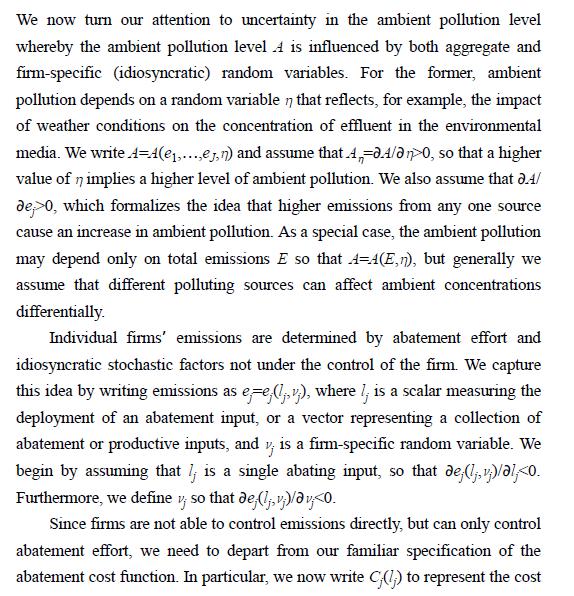
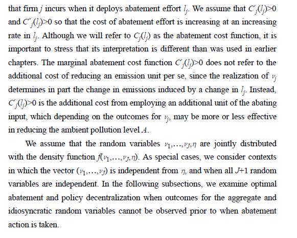
Data from section 9.2

Transcribed Image Text:

We now turn our attention to uncertainty in the ambient pollution level whereby the ambient pollution level 4 is influenced by both aggregate and firm-specific (idiosyncratic) random variables. For the former, ambient pollution depends on a random variable n that reflects, for example, the impact of weather conditions on the concentration of effluent in the environmental media. We write A=A(e,...,en) and assume that A-A/00, so that a higher value of n implies a higher level of ambient pollution. We also assume that d.4/ de 0, which formalizes the idea that higher emissions from any one source cause an increase in ambient pollution. As a special case, the ambient pollution may depend only on total emissions E so that A-A(E,n), but generally we assume that different polluting sources can affect ambient concentrations differentially. Individual firms' emissions are determined by abatement effort and idiosyncratic stochastic factors not under the control of the firm. We capture this idea by writing emissions as ee(lv), where ; is a scalar measuring the deployment of an abatement input, or a vector representing a collection of abatement or productive inputs, and v; is a firm-specific random variable. We begin by assuming that is a single abating input, so that delj, vj)/l; <0. Furthermore, we define v; so that de(lv)/@y <0. Since firms are not able to control emissions directly, but can only control abatement effort, we need to depart from our familiar specification of the abatement cost function. In particular, we now write C(l) to represent the cost