In Example 8.9 we estimated the linear probability model

where \(C O K E=1\) if a shopper purchased Coke and \(C O K E=0\) if a shopper purchased Pepsi. The variable PRATIO was the relative price ratio of Coke to Pepsi and DISP_COKE and DISP_PEPSI were indicator variables equal to one if the relevant display was present. Suppose now that we have 1140 observations on randomly selected shoppers from 50 different grocery stores. Each grocery store has its own settings for PRATIO,DISP_COKE and DISP_PEPSI. Let an \((i, j)\) subscript denote the \(j\) th shopper at the \(i\) th store, so that we can write the model as

Average this equation over all shoppers in the \(i\) th store so that we have

where

and \(N_{i}\) is the number of sampled shoppers in the \(i\) th store.

a. What is the interpretation of \(\overline{C O K E}_{i}\). for the \(i\) th store?

b. Assume that \(E\left(C O K E_{i j} \mid \mathbf{x}_{i j}\right)=P_{i}\) and \(\operatorname{var}\left(\operatorname{COKE_{ij}} \mid \mathbf{x}_{i j}\right)=P_{i}\left(1-P_{i}\right)\), show that \(E\left(\overline{\operatorname{COKE}}_{i} \cdot \mid \mathbf{X}\right)=\) \(P_{i}\) and \(\operatorname{var}\left(\overline{C O K E}_{i} \cdot \mid \mathbf{X}\right)=P_{i}\left(1-P_{i}\right) / N_{i}\).

d. Observations on the variables \(\overline{C O K E}_{i}\), PRATIO \({ }_{i}\), DISP_COKE \(_{i}, \overline{D I S P}_{-} \overline{P E P S I}_{i}\), and \(N_{i}\) appear in the data file coke_grouped. Obtain summary statistics for the data. Calculate the sample coefficient of variation, \(\mathrm{CV}=100 s_{x} / \bar{x}\), for \(\overline{C O K E}_{i}\). and \(P R A T I O_{i}\). How much variation is there in these variables relative to their mean? Would we prefer larger or smaller coefficients of variation in these variables? Why? Construct histograms for \(\overline{C O K E}_{i}\). and PRATIO\(_{i}\). What do you observe?

e. Find least squares estimates of equation (XR8.21) and use robust standard errors. Summarize the results. Test the null hypothesis \(\beta_{3}=-\beta_{4}\). Choose an appropriate alternative hypothesis and use the \(5 \%\) level of significance. If the null hypothesis is true, what does it imply about the effect of store displays for COKE and PEPSI?

f. Create the variable \(D I S P=D I S P_{-} C O K E-D I S P \_P E P S I\). Estimate the model \(\overline{C O K E}_{i}=\beta_{1}+\) \(\beta_{2}\) PRATIO \(_{i}+\beta_{3}\) DISP \(_{i}+\bar{e}_{i}\). by OLS. Test for heteroskedasticity by applying the White test. Also carry out the \(N R^{2}\) test for heteroskedasticity using the candidate variable \(N_{i}\). What are your conclusions, at the \(5 \%\) level?

g. Obtain the fitted values from (e), \(p_{i}\), and estimate \(\operatorname{var}\left(\overline{C O K E}_{i} \cdot\right)\) for each of the stores. Report the mean, standard deviation, maximum and minimum values of the \(p_{i}\).

h. Find generalized least squares estimates of the model in part (f). Comment on the results and compare them with those obtained in part (f). How might the results of part (d) help you?

Data From Example 8.9:-

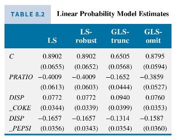
The choice of purchasing either Coke \((C O K E=1)\) or Pepsi \((C O K E=0)\) was modeled as depending on the relative price of Coke to Pepsi (PRATIO), and whether store displays for Coke and Pepsi were present (DISP_COKE = 1 if a Coke display was present, otherwise \(0 ; D I S P \_P E P S I=1\) if a Pepsi display was present, otherwise 0 ). The data file coke contains 1140 observations on these variables. Table 8.2 contains the results for (1) least squares, (2) least squares with robust standard errors, (3) GLS with variances below 0.01 truncated to 0.01 , and (4) GLS with observations not satisfying \(00.99\) and there were 16 observations where \(\hat{p}_{i}
Since the variance function in (8.32) contains the \(x\) ' \(s\), their squares, and their cross products, a suitable test for heteroskedasticity is the White test described in Section 8.6.4. Applying this test to the residuals from the least squares estimated equation yields

leading us to reject a null hypothesis of homoskedasticity at a \(1 \%\) level of significance. Note that, when carrying out this test, your software will omit the squares of DISP_COKE and DISP_PEPSI. Because these variables are indicator variables, \(D I S P_{-} C O K E^{2}=D I S P_{-} C O K E\) and \(D I S P_{-} P E P S I^{2}=\) \(D I S P \_P E P S I\), leaving a \(\chi^{2}\)-test with 7 degrees of freedom.
Examining the estimates in Table 8.2, we see there is little difference in the four sets of standard errors. In this particular case the use of least squares standard errors does not seem to matter. The four sets of coefficient estimates are

also similar with the exception of those from GLS where the negative \(\hat{p}\) 's were truncated to 0.01 . The weight on observations with variance \(\operatorname{var}\left(e_{i}\right)=0.01(1-0.01)=0.0099\) is a relatively large one. It appears that the large weights placed on those 16 observations are having a noticeable impact on the estimates. The signs are all as expected. Making Coke more expensive leads more people to purchase Pepsi. A Coke display encourages purchase of Coke, and a Pepsi display encourages purchase of Pepsi.
In Chapter 16 we study models which are specifically designed for modeling choice between two or more alternatives, and which do not suffer from the problems of the linear probability model.

Data From Equation 8.32:-

Transcribed Image Text:

COKE = B + BPRATIO+DISP_COKE + DISP_PEPSI + e