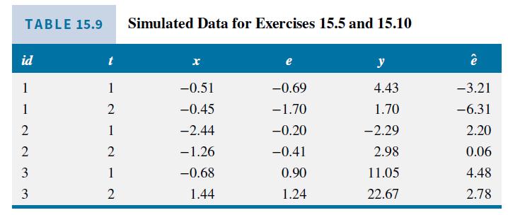
This exercise uses the simulated data (left(y_{i t}, x_{i t} ight)) in Table 15.9. a. The fitted least squares dummy variable model, given in equation

This exercise uses the simulated data \(\left(y_{i t}, x_{i t}\right)\) in Table 15.9.

a. The fitted least squares dummy variable model, given in equation (15.17), is \(\hat{y}_{i t}=5.57 D_{1 i}+\) \(9.98 D_{2 i}+14.88 D_{3 i}+5.21 x_{i t}\). Compute the residuals from this estimated model for \(i d=1\) and \(i d=2\). What pattern do you observe in these residuals?

b. The same residual pattern occurs for \(i d=3\). What is the correlation between the residuals for time periods \(t=1\) and \(t=2\) ?

c. The "within" model is given in equation (15.12). The transformed error is \(\tilde{e}_{i t}=\left(e_{i t}-\bar{e}_{i .}\right)\). If the assumptions FE1-FE5 hold, then \(\operatorname{var}\left(\tilde{e}_{i t}\right)=E\left[\left(e_{i t}-\bar{e}_{i \bullet}\right)^{2}\right]\), where \(\bar{e}_{i \cdot}=\left(e_{i 1}+e_{i 2}\right) / 2\) because \(T=2\). Show that \(\operatorname{var}\left(\tilde{e}_{i t}\right)=\sigma_{e}^{2} / 2\).

d. Using the same approach, as in part (c), show that \(\operatorname{cov}\left(\tilde{e}_{i 1}, \tilde{e}_{i 2}\right)=E\left[\left(e_{i 1}-\bar{e}_{i \text {. }}\right)\left(e_{i 2}-\bar{e}_{i \text {. }}\right)\right]=-\sigma_{e}^{2} / 2\).

e. Using the results in parts (c) and (d), it follows that \(\operatorname{corr}\left(\tilde{e}_{i 1}, \tilde{e}_{i 2}\right)=-1\). Relate this result to your answer in (b). In fact for \(T>1\), and assuming FE1-FE5 hold, \(\operatorname{corr}\left(\tilde{e}_{i t}, \tilde{e}_{i s}\right)=-1 /(T-1)\) if \(t eq s\). We anticipate the within-transformed errors to be serially correlated.

Data From Table 15.9:-

Data From Equation 15.17:-

TABLE 15.9 Simulated Data for Exercises 15.5 and 15.10 id t x y 1 -0.51 -0.69 4.43 -3.21 1 2 21212 233 -0.45 -1.70 1.70 -6.31 -2.44 -0.20 -2.29 2.20 -1.26 -0.41 2.98 0.06 -0.68 0.90 11.05 4.48 2 1.44 1.24 22.67 2.78