Question:
Use 200 observations from the Section 4.6.4 data on natural logarithm of health expenditure \((y)\) and natural logarithm of total expenditure \((x)\). Obtain OLS estimates of the model \(y=\alpha+\beta x+u\). Use the paired bootstrap with \(B=999\).
(a) Obtain a bootstrap estimate of the standard error of \(\widehat{\beta}\).
(b) Use this standard error estimate to test \(H_{0}: \beta=1\) against \(H_{a}: \beta eq 1\).
(c) Do a bootstrap test with refinement of \(H_{0}: \beta=1\) against \(H_{a}: \beta eq 1\) under the assumption that \(u\) is homoskedastic.
(d) If \(u\) is heteroskedastic what happens to your method in (c)? Is the test still asymptotically valid, and if so does it offer an asymptotic refinement?
(e) Do a bootstrap to obtain a bias-corrected estimate of \(\beta\).


Transcribed Image Text:
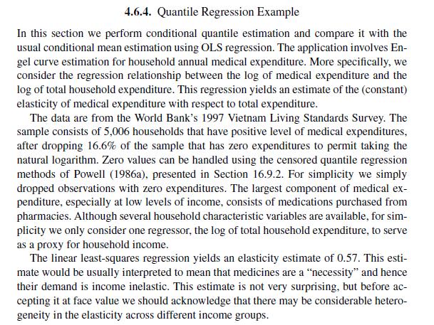
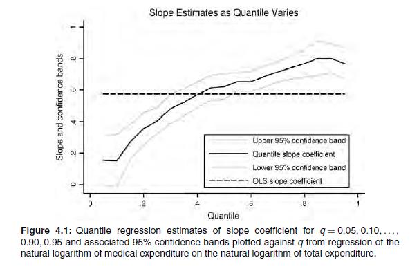
4.6.4. Quantile Regression Example In this section we perform conditional quantile estimation and compare it with the usual conditional mean estimation using OLS regression. The application involves En- gel curve estimation for household annual medical expenditure. More specifically, we consider the regression relationship between the log of medical expenditure and the log of total household expenditure. This regression yields an estimate of the (constant) elasticity of medical expenditure with respect to total expenditure. The data are from the World Bank's 1997 Vietnam Living Standards Survey. The sample consists of 5,006 households that have positive level of medical expenditures, after dropping 16.6% of the sample that has zero expenditures to permit taking the natural logarithm. Zero values can be handled using the censored quantile regression methods of Powell (1986a), presented in Section 16.9.2. For simplicity we simply dropped observations with zero expenditures. The largest component of medical ex- penditure, especially at low levels of income, consists of medications purchased from pharmacies. Although several household characteristic variables are available, for sim- plicity we only consider one regressor, the log of total household expenditure, to serve as a proxy for household income. The linear least-squares regression yields an elasticity estimate of 0.57. This esti- mate would be usually interpreted to mean that medicines are a "necessity" and hence their demand is income inelastic. This estimate is not very surprising, but before ac- cepting it at face value we should acknowledge that there may be considerable hetero- geneity in the elasticity across different income groups.
