1

2

3

4

5

6

7

8

9

10

11

12

13

14

15

16

17

18

19

20

21

22

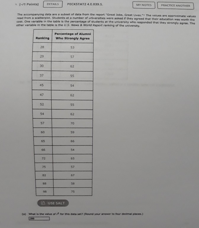
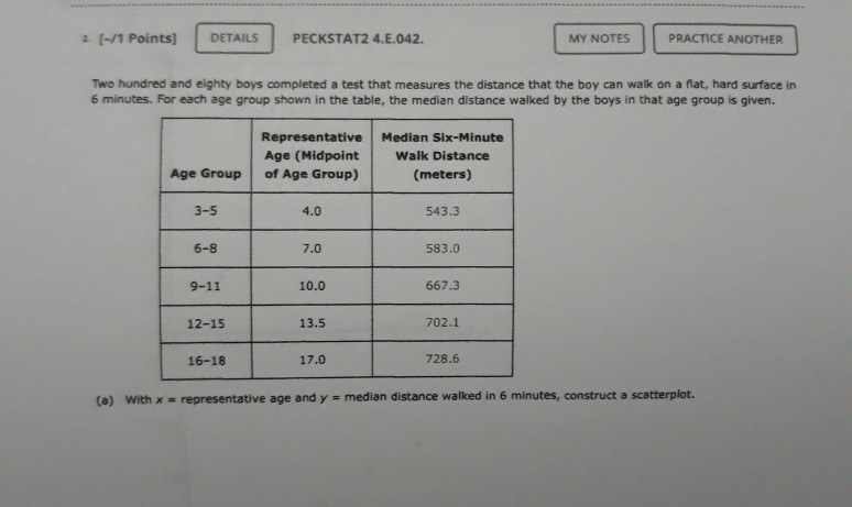
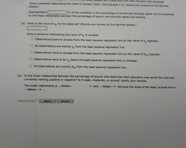
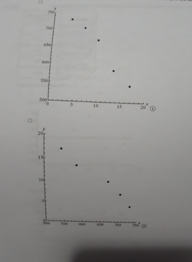
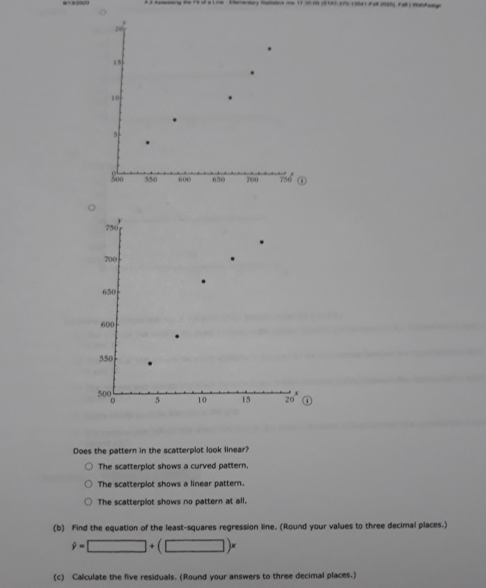
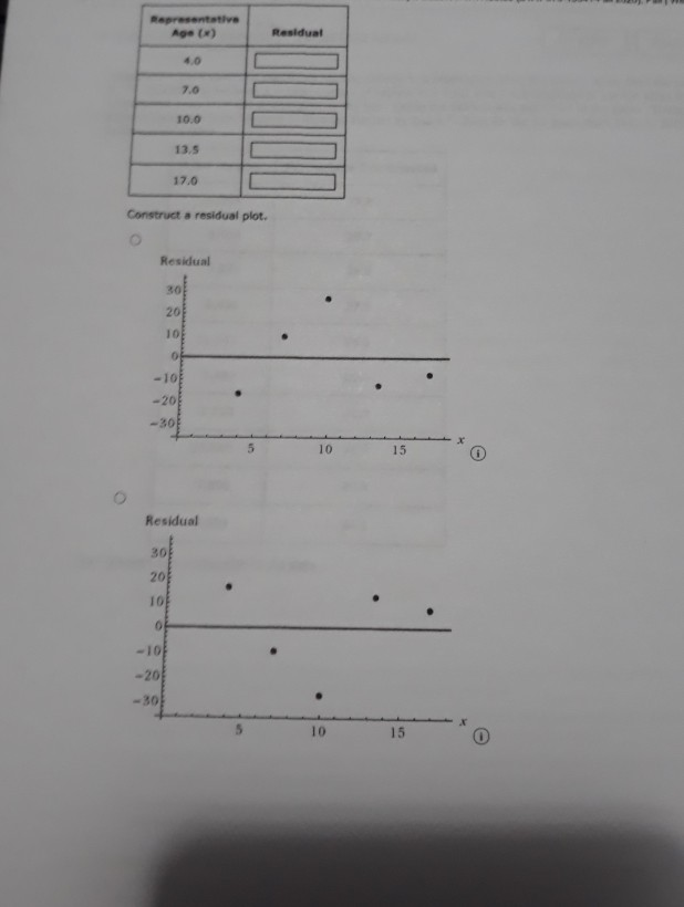
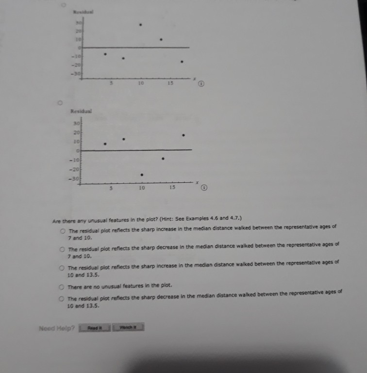
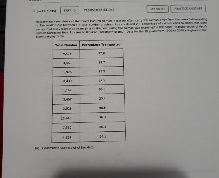
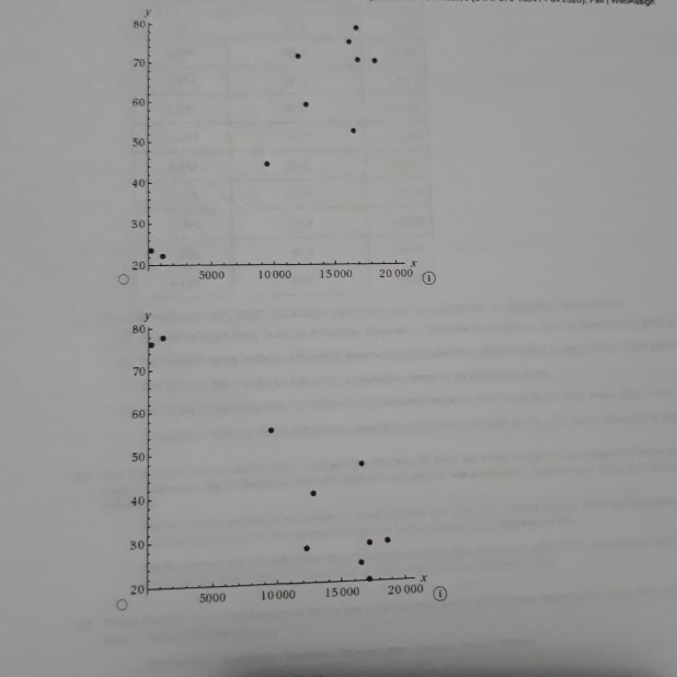
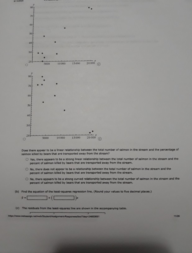
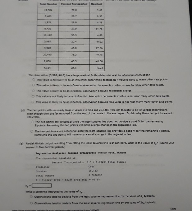
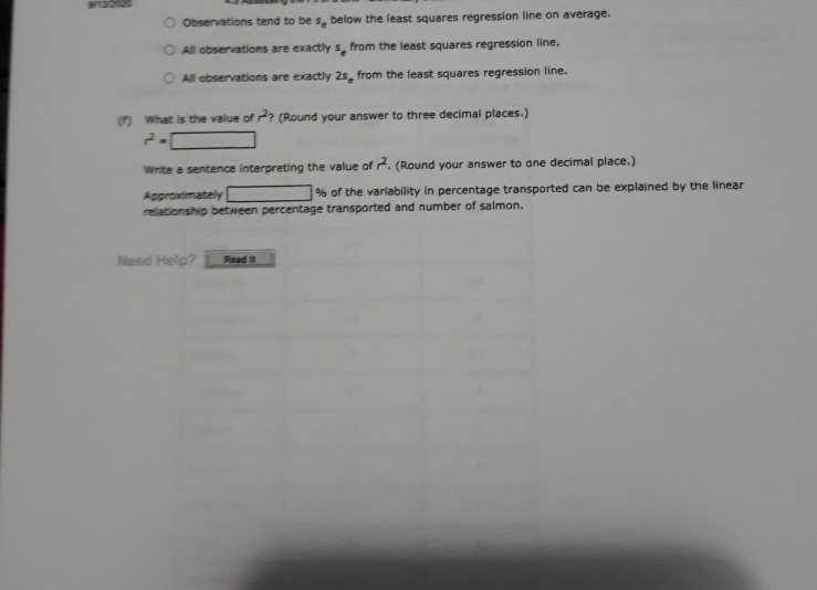
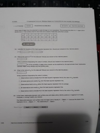
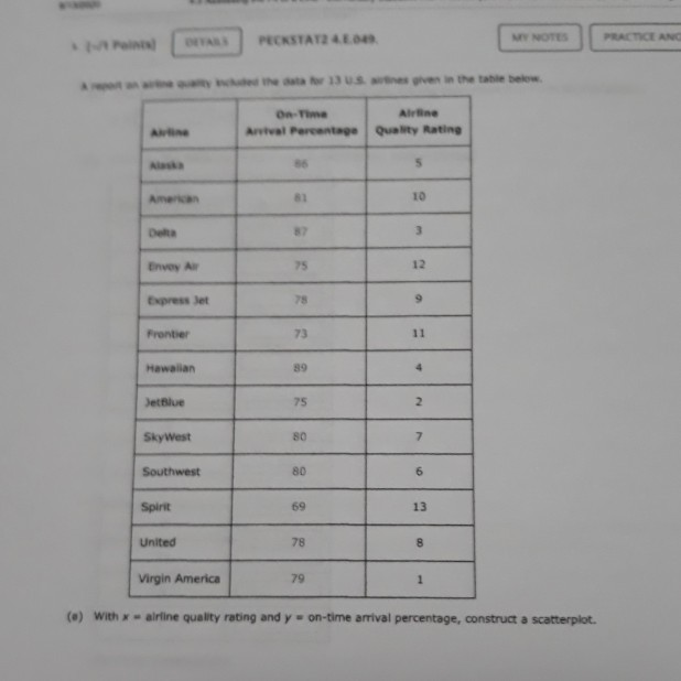
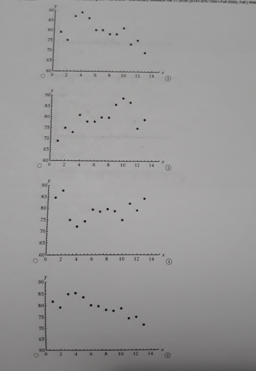
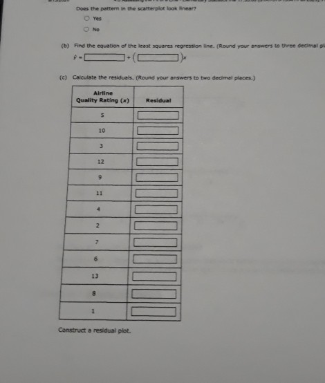
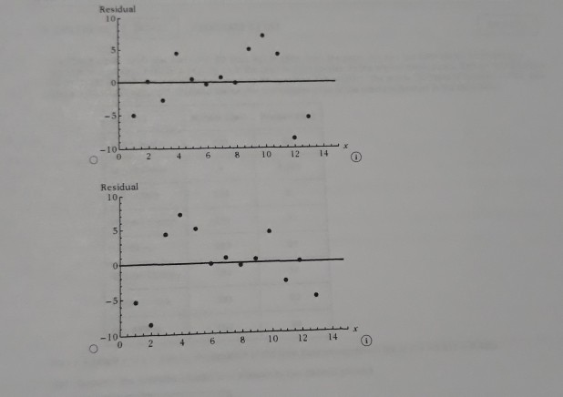
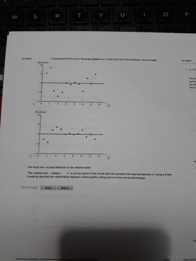
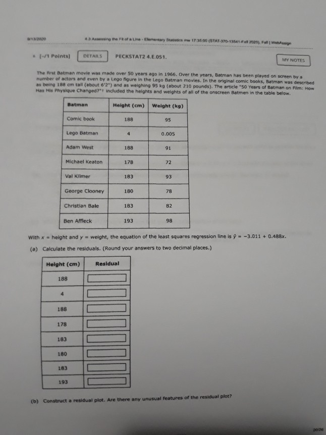
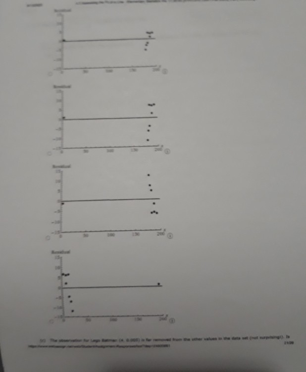
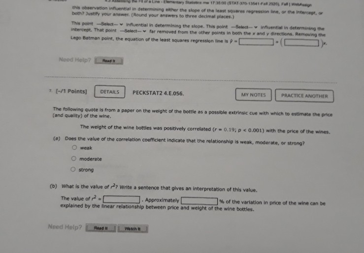
1 [-/1 Points) DETAILS PECKSTAT2 4.E.039.S. MY NOTES PRACTICE ANOTHER The accompanying data are a subset of data from the report "Great Jobs, Great Lives.*+ The values are approximate values read from a scatterplot. Students at a number of universities were asked if they agreed that their education was worth the cost. One variable in the table is the percentage of students at the university who responded that they strongly agree. The other variable in the table is the U.S. News & World Report ranking of the university. Percentage of Alumni Who Strongly Agree Ranking 28 53 29 57 30 62 37 55 45 54 47 62 52 55 54 62 57 70 60 59 65 66 66 54 72 65 75 57 82 67 88 58 98 75 A USE SALT (a) What is the value of for this data set? (Round your answer to four decimal places.) 286 2 (-/1 Points) DETAILS PECKSTAT2 4.E.042. MY NOTES PRACTICE ANOTHER Two hundred and eighty boys completed a test that measures the distance that the boy can walk on a flat, hard surface in 6 minutes. For each age group shown in the table, the median distance walked by the boys in that age group is given. Representative Age (Midpoint of Age Group) Median Six-Minute Walk Distance (meters) Age Group 3-5 4.0 543.3 6-8 7.0 583.0 9-11 10.0 667.3 12-15 13.5 702.1 16-18 17.0 728.6 (a) With x = representative age and y = median distance walked in 6 minutes, construct a scatterplot. (STAT-370-13541-Fall 2020). Fall WebAssign write a sentence interpreting this value in context. (Hint: See Example 4.13. Round your answer to two decimal places.) Approximately % of the variability in the percentage of alumni who strongly agree can be explained by the linear relationship between the percentage of alumni who strongly agree and ranking. (b) What is the value of s, for this data set? (Round your answer to five decimal places.) Write a sentence interpreting the value of se in context. Observations tend to deviate from the least squares regression line by the value of s typically. O All observations are exactly se from the least squares regression line. Observations tend to deviate from the least squares regression line by the value of 2s, typically. Observations tend to be s below the least squares regression line on average. All observations are exactly 2s, from the least squares regression line. (c) Is the linear relationship between the percentage of alumni who think that their education was worth the cost and university ranking positive or negative? Is it weak, moderate, or strong? Justify your answer. The linear relationship is ---Select--- and --Select---because the slope of the least squares line is --Select- Need Help? Read it Watch 730 700 650 600 550 500 5 10 15 20 15 10! Boo 500 700 750 Soo 350 750 750 700 650 600 550 500 0 10 15 20 O Does the pattern in the scatterplot look linear? The scatterplot shows a curved pattern. The scatterplot shows a linear pattern. The scatterplot shows no pattern at all. (b) Find the equation of the least-squares regression line. (Round your values to three decimal places.) - + (c) Calculate the five residuals. (Round your answers to three decimal places.) Representative Age Residual 4.0 7.0 10.0 13.5 17.0 Construct a residual plot. Residual 30 20 10 0 -10 -20 -30 10 15 Residual 201 10 01 -100 x 10 15 10 15 Residual 30 20 10 -10 - 203 -30 5 10 15 Are there any unusual features in the plot? (Hint: See Examples 4.6 and 4.7.) The residual plot reflects the sharp increase in the median distance walked between the representative ages of 7 and 10. The residual plot reflects the sharp decrease in the median distance walked between the representative ages of 7 and 10. The residual plot reflects the sharp increase in the median distance walked between the representative ages of 10 and 13.5. There are no unusual features in the plot. The residual plot reflects the sharp decrease in the median distance walked between the representative ages of 10 and 13.5. Need Help? Raad Watch MY NOTES (-/1 Points) PECKSTAT2 4.E.045. PRACTICE ANOTHER DETAILS Researchers have observed that bears hunting salmon in a creek often carry the salmon away from the creek before eating it. The relationship between x-total number of salmon in a creek and y-percentage of salmon killed by bears that were transported away from the stream prior to the bear eating the salmon was examined in the paper Transportation of Pacific Salmon Carcasses from Streams to Riparian Forests by Bears." + Data for the 10 years from 1999 to 2008 are given in the accompanying table. Total Number Percentage Transported 19,504 77.8 3,460 28.7 1,976 28.9 8,439 27.9 11,142 55.3 3,467 20.4 3,928 46.8 20,440 76.3 7,850 40.3 4,134 24.1 (a) Construct a scatterplot of the data. 170 16004 150 400 30 200 5000 10000 15000 20000 1800 170 600 500 400 301 2001 5000 10000 15000 20000 W2070 701 60 30 40 so Soon 10000 15000 20000 BO 70 60 50 40 30 20 5000 10000 15000 20 000 Does there appear to be a linear relationship between the total number of salmon in the stream and the percentage of salmon killed by bears that are transported away from the stream? O Yes, there appears to be a strong linear relationship between the total number of salmon in the stream and the percent of salmon killed by bears that are transported away from the stream. No, there does not appear to be a relationship between the total number of salmon in the stream and the percent of salmon killed by bears that are transported away from the stream. O No, there appears to be a strong curved relationship between the total number of salmon in the stream and the percent of salmon killed by bears that are transported away from the stream. (b) Find the equation of the least-squares regression line. (Round your values to five decimal places.) 9 - (c) The residuals from the least-squares line are shown in the accompanying table. www.webassin Student Assignment Responses/lastdep=24800661 Total Number Percent Transported Residual 77.8 3.43 0.30 1.975 28.9 -14.76 55.3 4.89 20.4 -8.02 3.928 46.8 17.06 20,440 76.3 -0.75 7,650 40.3 -0.68 4,134 24.1 -6.23 The observation (3,928, 46.8) has a large residual. Is this data point also an influential observation? This value is not likely to be an influential observation because its x value is close to many other data points. This value is likely to be an influential observation because its x value is close to many other data points. This value is likely to be an influential observation because its residual is large. This value is not likely to be an influential observation because its x value is not near many other data points. This value is likely to be an influential observation because its x value is not near many many other data points. The two points with unusually large x values (19,504 and 20,440) were not thought to be influential observations even though they are far removed from the rest of the points in the scatterplot. Explain why these two points are not influential The two points are influential since the least-squares line does not provide a good fit for the remaining 8 points. Removing the two points will make a large change in the regression line. The two points are not influential since the least-squares line provides a good fit for the remaining 8 points. Removing the two points will make only a small change in the regression line. (e) Partial Minitab output resulting from fitting the least-squares line is shown here. What is the value of s? (Round your answer to five decimal places.) Regression Analysis: Percent Transported versus Total Number The regression equation is Percent Transported - 18.5.0.00287 Total Number Predictor Coet Constant Total Bumber 0.0028655 5 - 9.16217 R-14 - 83.21 R-Sad) - 01.11 write a sentence interpreting the value of se Observations tend to deviate from the least squares regression line by the value of Se typically, Observations tend to deviate from the least squares regression line by the value of 2s, typically. infantil Observations tend to be s below the least squares regression line on average. All observations are exactly s from the least squares regression line, All observations are exactly 2s, from the least squares regression line. What is the value of 2 (Round your answer to three decimal places.) write a sentence interpreting the value of 2. (Round your answer to one decimal place.) Approximately % of the variability in percentage transported can be explained by the linear relationship between percentage transported and number of salmon. Need Help? Read CATATEME wapt to reme w of that come 4 USE SALT C wat in we color de Door de were De voor het ved wiring Od toron the water regione by the way Act 2, from the grein O tend to dever the quartetthet, mort, solarne There between there are web do te the relation --- PECKSTATE PEACTICE ANG Aline Artwal Percentage Quality Rating 5 American 10 3 Envoy A 25 12 Express Jet Frontier 11 Hawaiian JetBlue 75 2 SkyWest 80 7 Southwest 80 6 Spirit 69 13 United 78 8 Virgin America 79 1 ( ) with x airline quality rating and y - on-time arrival percentage, construct a scatterplot. 85 BO 70 65 10 12 90 85 80 751 701 651 60 8 10 12 14 90 851 80 75 70 65 60 6 8 10 12 14 90 85 80 75 70 65 60 10 12 14 Does the pattern in the scatterplot look linear? Yes NO () Find the equation of the least squares regression line. (Round your answers to three decimal - (c) Calculate the residuals. (Round your answers to two decimal places.) Airline Quality Rating (*) Residual 5 10 3 12 9 11 4 2 7 13 8 1 Construct a residual plot. Residual 100 -5 -10 10 12 Residual 100 5 -10 4 2 6 8 10 14 12 W E R T . The 10 Are there are features in the map The reserved that would be to the corres mee te desee the relationship bent ultrating in a rage 3 An the of an Elementary Staw 1735.00 (STAT-370-13541Fall 2020). FallWebAsign (-/1 Points) DETAILS PECKSTAT2 4.8.051. MY NOTES The first Batman movie was made over 50 years ago in 1966. Over the years, Batman has been played on screen by a number of actors and even by a lego figure in the Lego Batman movies. In the original comic books, Batman was described as being 188 cm tall (about 6'2") and as weighing 95 kg (about 210 pounds). The article "50 Years of Batman on Film: How Has His Physique Changed?"+ included the heights and weights of all of the onscreen Batmen in the table below. Batman Height (cm) Weight (kg) Comic book 188 95 Lego Batman 4 0.005 Adam West 188 91 Michael Keaton 178 72 Val Kilmer 183 93 George Clooney 180 78 Christian Bale 183 82 Ben Affleck 193 98 with x = height and y = weight, the equation of the least squares regression line is 9 = -3.011 +0.488x. (a) Calculate the residuals. (Round your answers to two decimal places.) Height (cm) Residual 188 4 188 178 183 180 183 193 (b) Construct a residual plot. Are there any unusual features of the residual plot? 3 1 Une Elementary Sam 17 00 (STAT-370-13541-Fall 2020). FallWeb this observation influential in determining either the slope of the least squares regression line, or the interceptor both? Justify your answer. (Round your answers to three decimal places.) This point -Select- influential in determining the slope. This point -Select influential in determining the Intercept. That point -Select- far removed from the other points in both the x and y directions. Removing the Lego Batman point, the equation of the least squares regression line is - Nood Help? Read 7. (-/1 Points] DETAILS PECKSTAT2 4.8.056. MY NOTES PRACTICE ANOTHER The following quote is from a paper on the weight of the bottle as a possible extrinsic cue with which to estimate the price (and quality) of the wine. The weight of the wine bottles was positively correlated (r=0.19; p