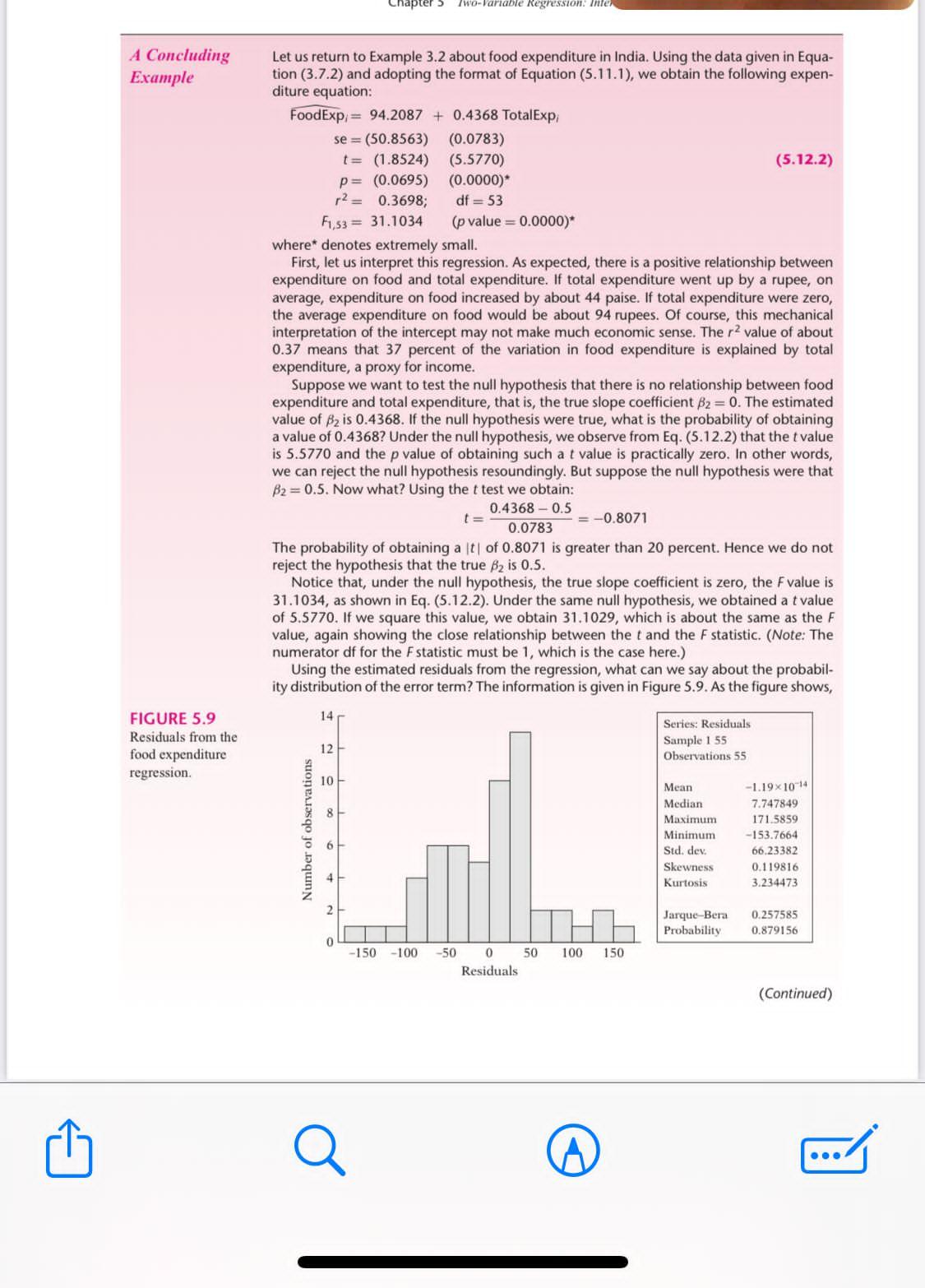
1 A Concluding Example FIGURE 5.9 Residuals from the food expenditure regression. Chapter 5 Two-Variable Regression: Inter Let us return to Example 3.2 about food expenditure in India. Using the data given in Equa- tion (3.7.2) and adopting the format of Equation (5.11.1), we obtain the following expen- diture equation: Food Exp, 94.2087 +0.4368 Total Exp se = (50.8563) (0.0783) t = (1.8524) (5.5770) p = (0.0695) (0.0000)* r = 0.3698; df=53 (5.12.2) F1,53 = 31.1034 (p value=0.0000)* where* denotes extremely small. First, let us interpret this regression. As expected, there is a positive relationship between expenditure on food and total expenditure. If total expenditure went up by a rupee, on average, expenditure on food increased by about 44 paise. If total expenditure were zero, the average expenditure on food would be about 94 rupees. Of course, this mechanical interpretation of the intercept may not make much economic sense. The r2 value of about 0.37 means that 37 percent of the variation in food expenditure is explained by total expenditure, a proxy for income. Suppose we want to test the null hypothesis that there is no relationship between food expenditure and total expenditure, that is, the true slope coefficient B2 = 0. The estimated value of B is 0.4368. If the null hypothesis were true, what is the probability of obtaining a value of 0.4368? Under the null hypothesis, we observe from Eq. (5.12.2) that the t value is 5.5770 and the p value of obtaining such a t value is practically zero. In other words, we can reject the null hypothesis resoundingly. But suppose the null hypothesis were that B2=0.5. Now what? Using the t test we obtain: t= 0.4368-0.5 0.0783 = -0.8071 The probability of obtaining a |t| of 0.8071 is greater than 20 percent. Hence we do not reject the hypothesis that the true B is 0.5. Notice that, under the null hypothesis, the true slope coefficient is zero, the F value is 31.1034, as shown in Eq. (5.12.2). Under the same null hypothesis, we obtained a t value of 5.5770. If we square this value, we obtain 31.1029, which is about the same as the F value, again showing the close relationship between the t and the F statistic. (Note: The numerator df for the F statistic must be 1, which is the case here.) Using the estimated residuals from the regression, what can we say about the probabil- ity distribution of the error term? The information is given in Figure 5.9. As the figure shows, Number of observations 14 12 10 8 Series: Residuals Sample 1 55: Observations 55 Mean Median -1.19x10 14 7.747849 171.5859 -153.7664 Maximum Minimum Std. dev. Skewness Kurtosis 66.23382 0.119816 3.234473 -150 -100 -50 0 Residuals 50 100 150 Jarque-Bera 0.257585 Probability. 0.879156 (Continued)