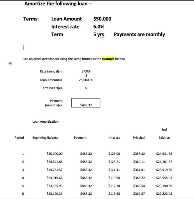
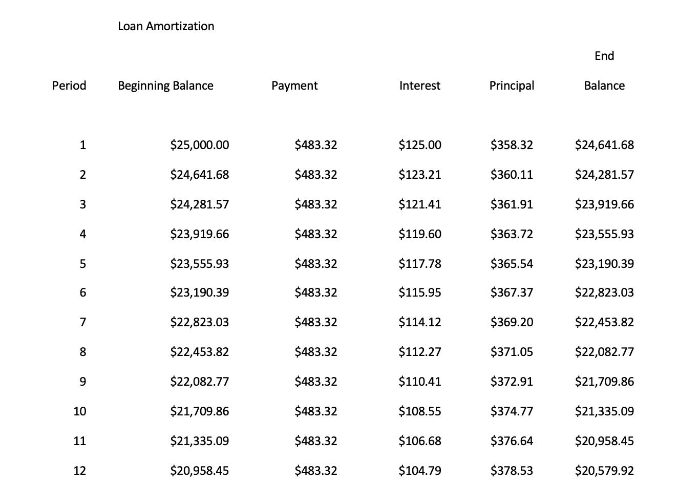
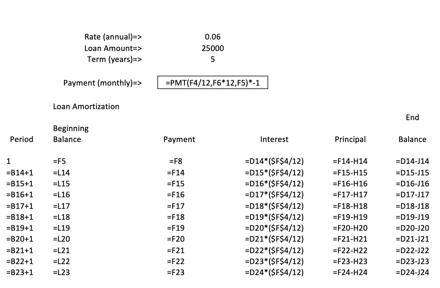
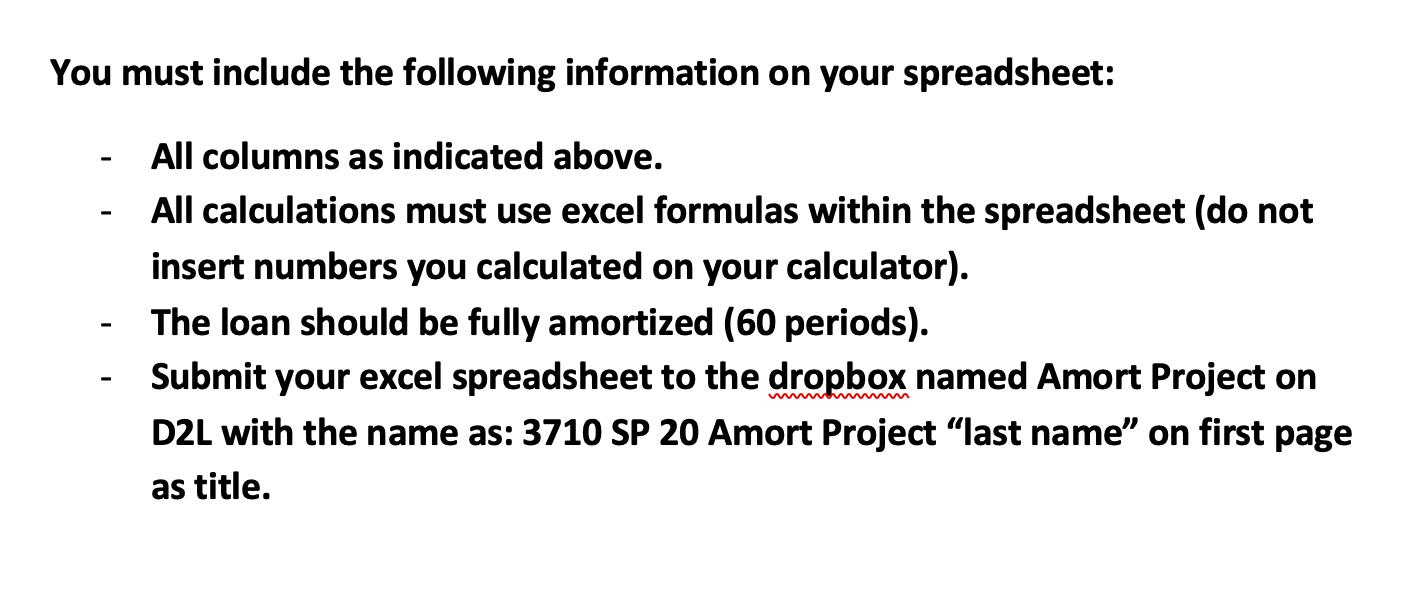
+ Terms: I Period 1 use an excel spreadsheet using the same format as the example below: 2 Amortize the following loan -- 3 4 5 6 Loan Amount Interest rate Term Rate (annual) => Loan Amount=> Term (years)=> Payment (monthly)=> Loan Amortization Beginning Balance $25,000.00 $24,641.68 $24,281.57 $23,919.66 $23,555.93 $23,190.39 6.00% $ 25,000.00 5 $483.32 Payment $483.32 $50,000 6.0% 5 yrs Payments are monthly $483.32 $483.32 $483.32 $483.32 $483.32 Interest $125.00 $123.21 $121.41 $119.60 $117.78 $115.95 Principal $358.32 $360.11 $361.91 $363.72 $365.54 $367.37 End Balance $24,641.68 $24,281.57 $23,919.66 $23,555.93 $23,190.39 $22,823.03 Period 1 2 3 4 5 6 7 8 9 10 11 12 Loan Amortization Beginning Balance $25,000.00 $24,641.68 $24,281.57 $23,919.66 $23,555.93 $23,190.39 $22,823.03 $22,453.82 $22,082.77 $21,709.86 $21,335.09 $20,958.45 Payment $483.32 $483.32 $483.32 $483.32 $483.32 $483.32 $483.32 $483.32 $483.32 $483.32 $483.32 $483.32 Interest $125.00 $123.21 $121.41 $119.60 $117.78 $115.95 $114.12 $112.27 $110.41 $108.55 $106.68 $104.79 Principal $358.32 $360.11 $361.91 $363.72 $365.54 $367.37 $369.20 $371.05 $372.91 $374.77 $376.64 $378.53 End Balance $24,641.68 $24,281.57 $23,919.66 $23,555.93 $23,190.39 $22,823.03 $22,453.82 $22,082.77 $21,709.86 $21,335.09 $20,958.45 $20,579.92 Period 1 =B14+1 =B15+1 =B16+1 =B17+1 =B18+1 =B19+1 =B20+1 =B21+1 =B22+1 =B23+1 Rate (annual)=> Loan Amount => Term (years) => Payment (monthly)=> Loan Amortization Beginning Balance =F5 =L14 =L15 =L16 =L17 =L18 =L19 =L20 =L21 =L22 =L23 =PMT(F4/12,F6*12, F5)*-1 Payment 0.06 25000 5 =F8 =F14 =F15 =F16 =F17 =F18 =F19 =F20 =F21 =F22 =F23 Interest =D14* ($F$4/12) =D15*($F$4/12) =D16*($F$4/12) =D17*($F$4/12) =D18*($F$4/12) =D19* ($F$4/12) =D20* ($F$4/12) =D21*($F$4/12) =D22* ($F$4/12) =D23* ($F$4/12) =D24*($F$4/12) Principal =F14-H14 =F15-H15 =F16-H16 =F17-H17 =F18-H18 =F19-H19 =F20-H20 =F21-H21 =F22-H22 =F23-H23 =F24-H24 End Balance =D14-J14 =D15-J15 =D16-J16 =D17-J17 =D18-J18 =D19-J19 =D20-J20 =D21-J21 =D22-J22 =D23-J23 =D24-J24 You must include the following information on your spreadsheet: All columns as indicated above. All calculations must use excel formulas within the spreadsheet (do not insert numbers you calculated on your calculator). The loan should be fully amortized (60 periods). Submit your excel spreadsheet to the dropbox named Amort Project on D2L with the name as: 3710 SP 20 Amort Project "last name" on first page as title. -