1. for a single wire, we need a plot of the voltage drop across a segment of wire (V ) as a function of the length of

that segment of wire (l).

2. a plot of voltage drop across the entire wire (V ) as a function of current (I) through the wire, for each wire.

This should include a minimum of 5 different current values. This should demonstrate that each wire is an Ohmic

material (i.e., it behaves Ohm's law).

3. a table of the values and uncertainties measured for the resistance, R, the diameter, d, and the

length, l, of each wire. From those, compute the resistivity, , of each wire and propagate the uncertainty. An example

table is shown in Section 5.

4. a description of the process used to measure the values and uncertainties for R, d, and l in the previous

table.

5. assessment of each wire's composition based on your resistivity values

All the datas can be find here :

-Voltage_curent_data :

v_vs_i_wire_1 :

Current	Voltage
0.1	0.608
0.09	0.547
0.08	0.487
0.07	0.425
0.06	0.364
0.05	0.304
0.04	0.242
0.03	0.181
0.02	0.121
0.01	0.058

v_vs_i_wire_2

Current	Voltage
0.1	0.948
0.09	0.854
0.08	0.759
0.07	0.662
0.06	0.568
0.05	0.473
0.04	0.376
0.03	0.281
0.02	0.187
0.01	0.089

v_vs_i_wire_3

Current	Voltage
0.1	1.562
0.09	1.407
0.08	1.251
0.07	1.091
0.06	0.935
0.05	0.78
0.04	0.619
0.03	0.464
0.02	0.308
0.01	0.148

-Voltage_lenght_data :

v_vs_l_wire_1 :

Applied length (mm)	Chnl. 0 (V)	Chnl. 0 uncert. (V)
0.0	0.005923828125	0.0009736595740586162
50.0	0.0468837890625	0.0010745324999020002
100.0	0.089900390625	0.0010988140631737777
150.0	0.132298828125	0.001095746348788153
200.0	0.172775390625	0.0010241062994708933
250.0	0.2162607421875	0.0010568074032074437
300.0	0.2597314453125	0.0010701983425769864
350.0	0.2993876953125	0.0010459539072409897
400.0	0.3417802734375	0.0009915080522796024
450.0	0.3846005859375	0.0010530434411046177
500.0	0.42491015625	0.001084707465750505
550.0	0.4713193359375	0.0010693795648741595
600.0	0.50947265625	0.0010809395581479755
650.0	0.552017578125	0.0010157692411845666

v_vs_l_wire_2 :

Applied length (mm)	Chnl. 0 (V)	Chnl. 0 uncert. (V)
0	0.008765625	0.000931806
50	0.06890625	0.00120958
100	0.139643555	0.001004771
150	0.205555664	0.001028952
200	0.27290625	0.001071404
250	0.339594727	0.000987725
300	0.406256836	0.00106675
350	0.475353516	0.00104188
400	0.539182617	0.000969967
450	0.60431543	0.001079058
500	0.672269531	0.001042997
550	0.737414063	0.001001244
600	0.803953125	0.001090359
650	0.869214844	0.00107976

v_vs_l_wire_3 :

Applied length (mm)	Chnl. 0 (V)	Chnl. 0 uncert. (V)
0.0	0.0088212890625	0.0009435544201631983
50.0	0.116947265625	0.0010576994590144053
100.0	0.223078125	0.0010446596195427128
150.0	0.33540234375	0.0009909610868911159
200.0	0.44537109375	0.001046762215531425
250.0	0.5584833984375	0.000984694767921814
300.0	0.667400390625	0.0010740985710473354
350.0	0.7779375	0.001065515317222306
400.0	0.887724609375	0.0010156424183452258
450.0	0.9986337890625	0.0010685021002520786
500.0	1.108271484375	0.0009923898565638853
550.0	1.221509765625	0.001070722169758912
600.0	1.325701171875	0.0010334115585333382
650.0	1.4398916015625	0.0010228919514287864

Wire_measurements :

Overall wire length:

l = 705 5 mm

Wire 1 diameter:

d1 = 0.42 0.01 mm

Wire 2 diameter:

d2 = 0.34 0.01 mm

Wire 3 diameter:

d3 = 0.27 0.01 mm

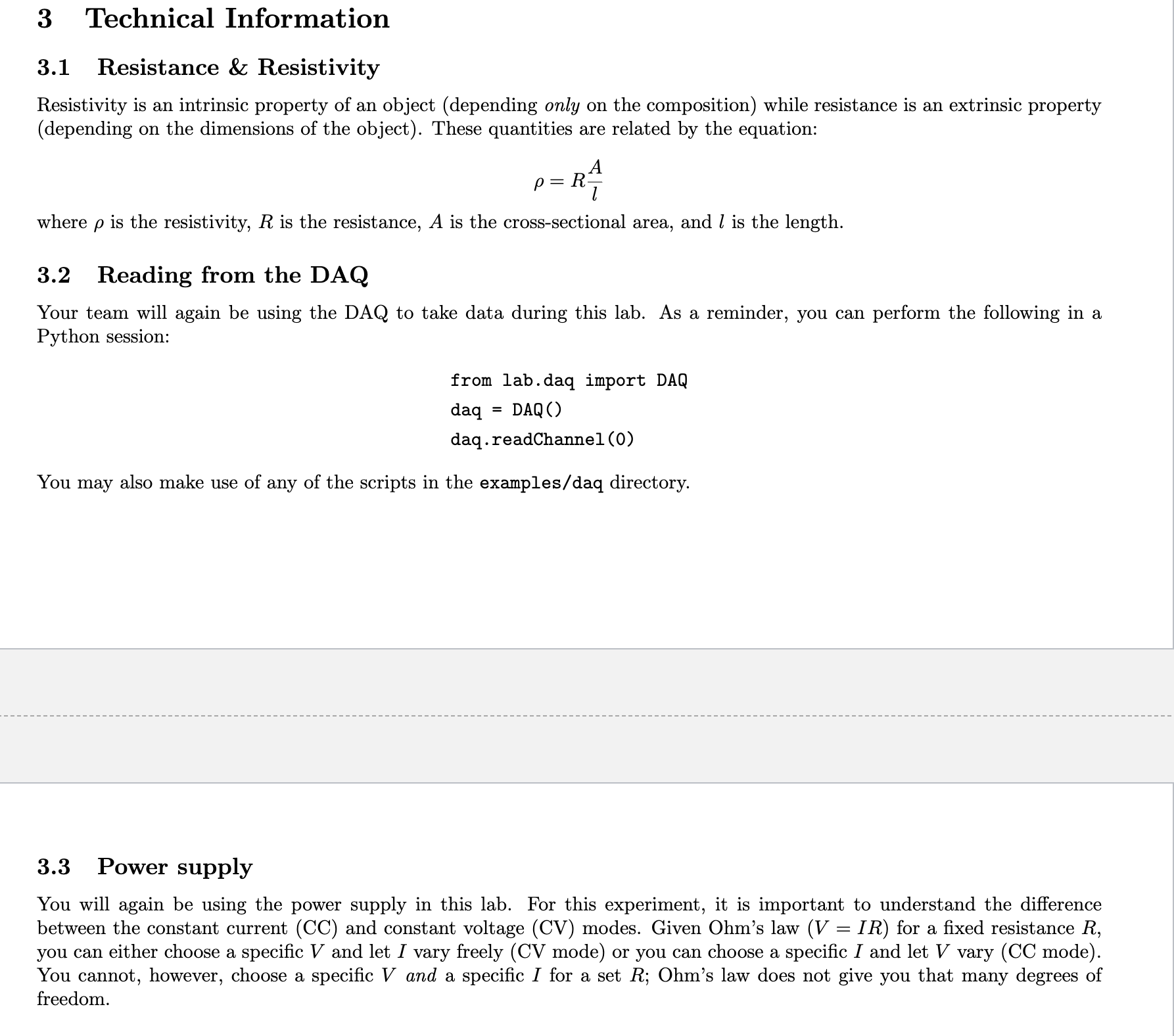
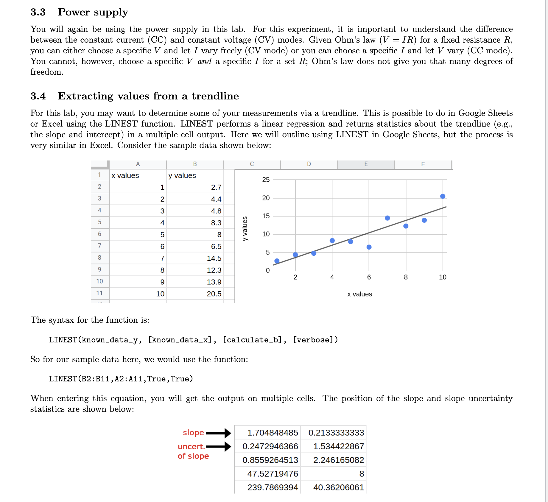
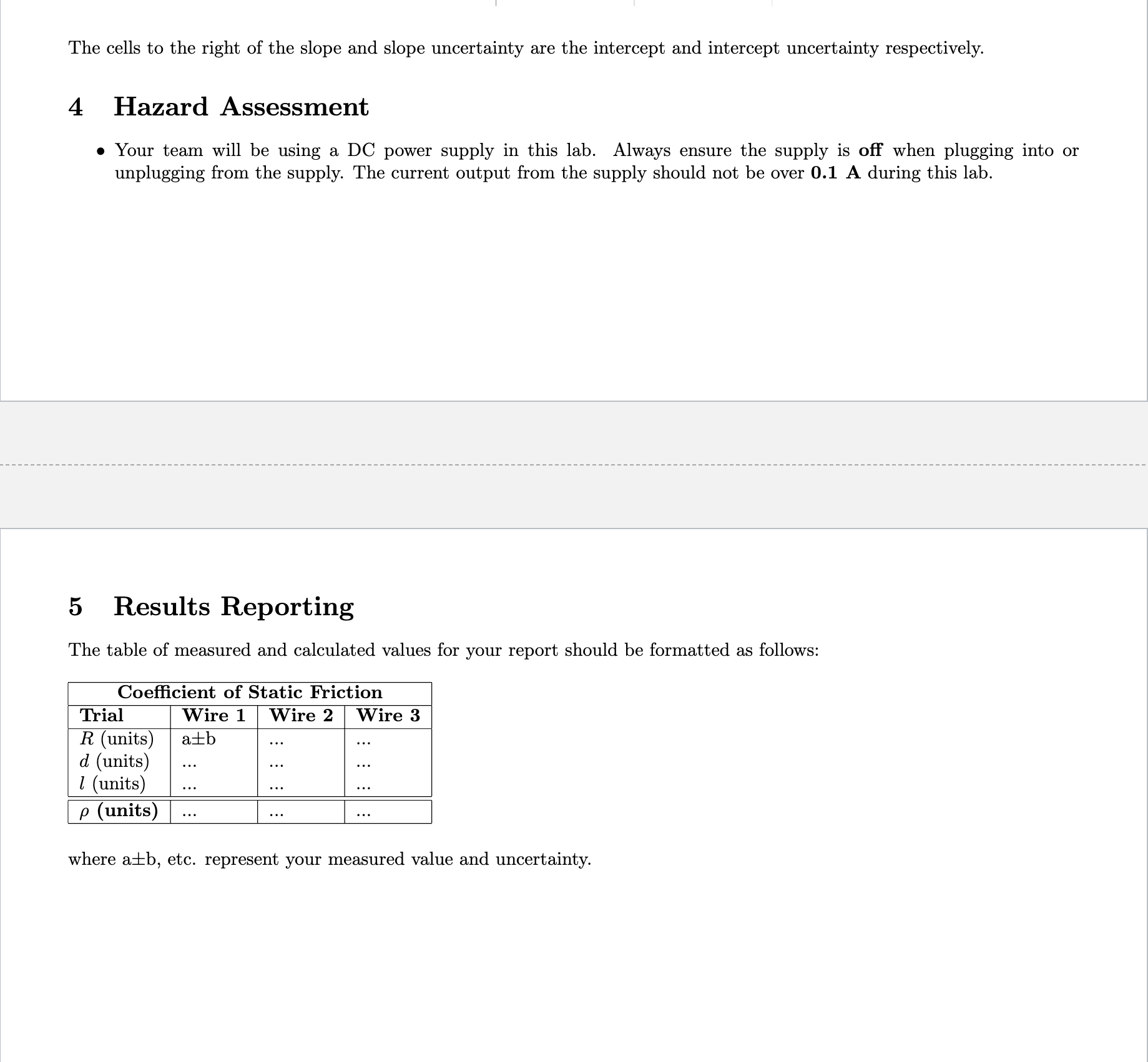
3 Technical Information 3.1 Resistance & Resistivity Resistivity is an intrinsic property of an object (depending only on the composition) while resistance is an extrinsic property (depending on the dimensions of the object). These quantities are related by the equation: A '0_RT where p is the resistivity, R is the resistance, A is the cross-sectional area, and l is the length. 3.2 Reading from the DAQ Your team will again be using the DAQ to take data during this lab. As a reminder, you can perform the following in a Python session: from lab.daq import DAD daq = DAQO daq . readCharmel (0) You may also make use of any of the scripts in the examples/daq directory. 3.3 Power supply You will again be using the power supply in this lab. For this experiment, it is important to understand the difference between the constant current (CC) and constant voltage (CV) modes. Given Ohm's law (V 2 IR) for a xed resistance R, you can either choose a specic V and let I vary freely (CV mode) or you can choose a specic I and let V vary (CC mode). You cannot, however, choose a specic V and a specic I for a set R; Ohm's law does not give you that many degrees of freedom. 3.3 Power supply You will again be using the power supply in this lab. For this experiment, it is important to understand the difference between the constant current (CC) and constant voltage (CV) modes. Given Ohm's law (V = IR) for a fixed resistance R, you can either choose a specific V and let I vary freely (CV mode) or you can choose a specific I and let V vary (CC mode). You cannot, however, choose a specific V and a specific I for a set R; Ohm's law does not give you that many degrees of freedom. 3.4 Extracting values from a trendline For this lab, you may want to determine some of your measurements via a trendline. This is possible to do in Google Sheets or Excel using the LINEST function. LINEST performs a linear regression and returns statistics about the trendline (e.g., the slope and intercept) in a multiple cell output. Here we will outline using LINEST in Google Sheets, but the process is very similar in Excel. Consider the sample data shown below: B C D E 1 x values y values 25 2 1 2.7 3 4.4 20 4 w 4.8 15 5 4 8.3 y values 6 5 8 10 7 6 6.5 5 8 7 14.5 9 8 12.3 10 4 6 8 10 13.9 2 11 10 20.5 x values The syntax for the function is: LINEST (known_data_y, [known_data_x] , [calculate_b], [verbose]) So for our sample data here, we would use the function: LINEST (B2 : B11 , A2 : A11, True, True) When entering this equation, you will get the output on multiple cells. The position of the slope and slope uncertainty statistics are shown below: slope 1.704848485 0.2133333333 uncert 0.2472946366 1.534422867 of slope 0.8559264513 2.246165082 47.52719476 8 239.7869394 40.36206061The cells to the right of the slope and slope uncertainty are the intercept and intercept uncertainty respectively. 4 Hazard Assessment 0 Your team will be using a DC power supply in this lab. Always ensure the supply is off when plugging into or unplugging from the supply. The current output from the supply should not be over 0.1 A during this lab. 5 Results Reporting The table of measured and calculated values for your report should be formatted as follows: Coefcient of Static Friction Trial Wire 1 Wire 2 Wire 3 R (units) azlzb (1 (units) 1! (units) p (units) l where a:|:b, etc. represent your measured value and uncertainty