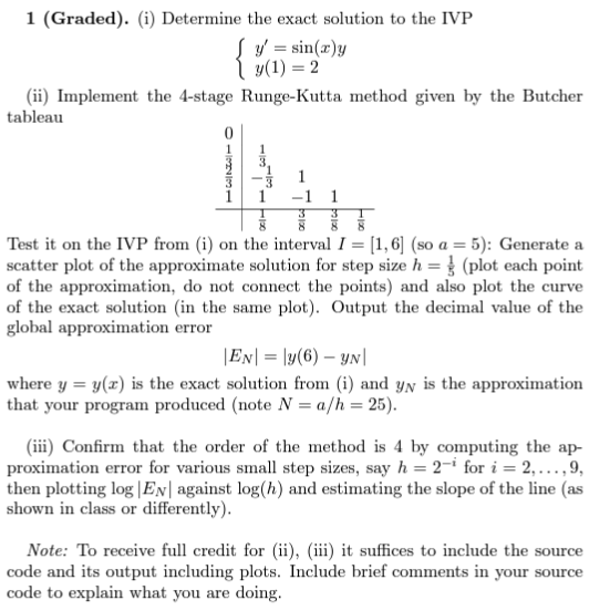
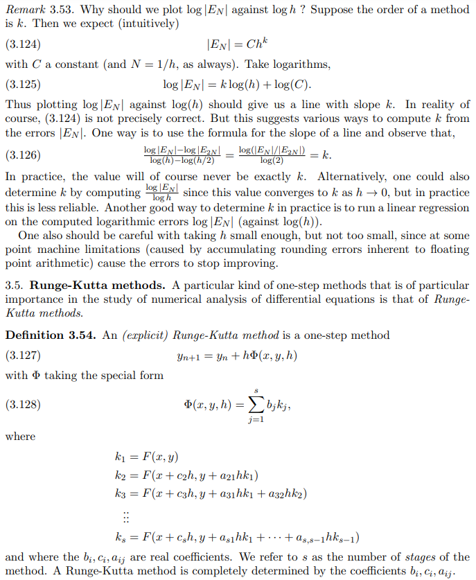
1 (Graded). (i) Determine the exact solution to the IVP y' = sin(r)y i y(1) = 2 (ii) Implement the 4-stage Runge-Kutta method given by the Butcher tableau -1 Test it on the IVP from (i) on the interval / = [1, 6] (so a = 5): Generate a scatter plot of the approximate solution for step size h = (plot each point of the approximation, do not connect the points) and also plot the curve of the exact solution (in the same plot). Output the decimal value of the global approximation error |ENI = ly(6) - yN| where y = y(x) is the exact solution from (i) and ya is the approximation that your program produced (note N = a/h = 25). (iii) Confirm that the order of the method is 4 by computing the ap- proximation error for various small step sizes, say h = 2- for i = 2,...,9, then plotting log | Ev| against log(h) and estimating the slope of the line (as shown in class or differently). Note: To receive full credit for (ii), (iii) it suffices to include the source code and its output including plots. Include brief comments in your source code to explain what you are doing.[B] J. C. Butcher. General Linear Methods. Acta Numerica 15 (2006), 157-256. [RS] J. Roos, A. Seeger. Analysis II. Lecture notes. https:/ /faculty.uml.edu/joris_roos/files/522.pdf SM] E. Suli, D. Mayers. An Introduction to Numerical Analysis, Cambridge University Press H P. Hartman. Ordinary differential equations. D. G. Zill. A first course in differential equations, with modeling applications. Ninth editionRemark 3.53. 'Nhy should we plot log |EN| against log I). ? Suppose the order of a method is k. Then we expect. {intuitively} {3.124) |EN| = Chi with C a constant (and N = lfln as always). Take logarithms: {3.125) log|EN| = klog(l1)+log(C}. Thus plotting log|EN| against log(h) should give us a line with slope k. In reality of course, (3.124) is not precisely correct. But this suggests various ways to compute is from the errors |EN|. One way is to use the formula for the slope of a line and observe that, bsth-losihl _ 103(2) In practice, the value will of course never be exactly k. Alternatively, one could also determine 1:: by computing half}? I since this value converges to k as h > 0.. but. in practice this is less reliable. Another good way to determine k in practice is to run a linear regression on the computed logarithmic errors log |EN| {against log(Ii}). One also should be careful with taking it small enough. but not too small. since at some point machine limitations (caused by accumulating rounding errors inherent to oating point arithmetic) cause the errois to stop improving. {3.126) loleml-loalEml IDEUENIJ'IEMIIJ = h 3.5. Runge-Kutta methods. A particular kind of one-step methods that is of particular importance in the study of numerical analysis of differential equations is that of Range K-utta methods. Denition 3.54. An (explicit) Range-Katie: method is a onestep method (3.12?) yin-+1 : y + h(n, y: h) with I1) taking the special form (3.12s) spay. h) = 2 his}. 3'21 where 531 = Fix: ii} k2 = PM + egh, y + agglhkl) k3 = Fi: + (sh, 3,: + aslhfcl + asahkal ks 2 PM + csh1 y + trufe] + - - - + asrslhksl) and where the 5;, ch HU are real coefficients. TWe refer to s as the number of stages of the method. A RungeKutta method is completely determined by the coefcients bi. cmaij. Runge-Kutta methods are often visualized using a Butcher tableau: C2 031 032 (3.129) (8,8-1 b1 b2 Example 3.55. Euler's method (s = 1), the midpoint method (s = 2) and Heun's method (s = 2) are explicit Runge-Kutta methods that can be represented by Butcher tableaus: (3.130) Example 3.56. Method (C) from Exercise 3.52 is a 3-stage Runge-Kutta method represented by the Butcher tableau (3.131) wi- 0 As we have seen in Exercise 3.52, this method has order 3. (Whereas the method (D), which is also a consistent 3-stage Runge-Kutta method only has order 1.) Example 3.57. The classical Runge-Kutta method of order 4 (also known as RK4) is the 4-stage Runge-Kutta method given by HNIHI- (3.132) GI- O O N1- The ease of implementation and high accuracy of this method have made it very popular in practical applications. Exercise 3.58. Implement this 4-stage Runge-Kutta method and confirm empirically using the initial value problems from Exercises 3.38 and 3.52 that is has order 4. From Fact 3.45 we see that a Runge-Kutta method is consistent if and only if (3.133) [bj = 1. j=1 Consistent Runge-Kutta methods have at least order 1. Note carefully that the order of an s-stage Runge-Kutta is not necessarily given by s. It is not obvious at all how to chooseS 4 S = K 11 29 TABLE 1. Minimum number of stages s for an explicit Runge-Kutta method of order k [B]. For large & the answer is not known. the coefficients bi, G, a so that the resulting method has a large order. In fact, it is an unsolved problem to determine for a given & what the minimum value of s is so that there exists an s-stage Runge-Kutta method of order k. For k 2 5 it is well-known that s > k is necessary (see Butcher [B]). Determining the order of a given Runge-Kutta method is typically achieved by analyzing the truncation error (3.112) using appropriate Taylor expansion. Exercise 3.59. (i) Write down the Butcher tableau and the map & for a general 2-stage Runge-Kutta method. (ii) Determine all 2-stage Runge-Kutta methods of order at least 1. (ini*) Determine all 2-stage Runge-Kutta methods of order 2. Solution (*). (i) (3.134) (3.135) D(r, y, h) = biF(x, y) + b2F(x + ch, y + ahF(x, y)). (ii) A method has order at least 1 if and only if it is consistent. Thus we need by + by = 1. The values of c, a are arbitrary. (iii*) We need to study the truncation error (3.136) In = H(y(In th) - y(In)) - D(In, y(1, ), h). By Taylor's theorem we have (3.137) y(In th) = y(In) +hy'(In ) + hay"(In) + O(h3). Here O(h3) is the usual "Big-O" notation: it is a placeholder for an "error term" that is bounded by a constant times " in absolute value. With this we have (3.138) In = y'(In) + hy"(In) - D(In, y(In), h) + O(h?)Let us introduce some abbreviations for the rest of this computation: (3.139) *= In, y = y(In), y' = y'(In), y" = y"(In), F = F(In, yn) (whenever we use arguments evaluated at 2 = T, then arguments are omitted from nota- tion) Then substituting the definition of , (3.140) In = y' t thy" - bF - bF(x + ch,y + ahF) + O(h?) To analyze this further we notice that by the ODE, (3.141) y = F and by the chain rule, (3.142) y" = OF + y'dF = OF + FoyF. For a smooth function F of two variables we have by the two-dimensional Taylor formula: (3.143) F(a + Ar, y + Ay) = F(x, y) + Ard.F(x, y) + Ayo, F(x,y) + O(h2), whenever |Ar| + [Ay)