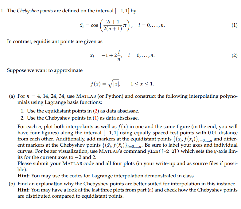
1. The Chebyshev points are defined on the interval [-1,1] by 2i+1 In contrast, equidistant points are given as Xi =-1 + 2-, 1-0, ,n. Suppose we want to approximate (a) For n -4, 14, 24, 34, use MATLAB (or Python) and construct the following interpolating polyno- mials using Lagrange basis functions 1. Use the equidistant points in (2) as data abscissae 2. Use the Chebyshev points in (1) as data abscissae For each n, plot both interpolants as well as f (x) in one and the same figure (in the end, you will have four figures) along the interval [-1,1] using equally spaced test points with 0.01 distance from each other. Additionally, add markers at the equidistant points {(xi, (xi))i-0 n and differ- ent markers at the Chebyshev points (t,, f(ti..Be sure to label your axes and individual curves. For better visualization, use MATLAB's command ylim([-2 2]) which sets the y-axis lim- its for the current axes to-2 and 2 Please submit your MATLAB code and all four plots (in your write-up and as source files if possi- ble) Hint: You may use the codes for Lagrange interpolation demonstrated in class. (b) Find an explanation why the Chebyshev points are better suited for interpolation in this instance Hint: You may have a look at the last three plots from part (a) and check how the Chebyshev points are distributed compared to equidistant points. 1. The Chebyshev points are defined on the interval [-1,1] by 2i+1 In contrast, equidistant points are given as Xi =-1 + 2-, 1-0, ,n. Suppose we want to approximate (a) For n -4, 14, 24, 34, use MATLAB (or Python) and construct the following interpolating polyno- mials using Lagrange basis functions 1. Use the equidistant points in (2) as data abscissae 2. Use the Chebyshev points in (1) as data abscissae For each n, plot both interpolants as well as f (x) in one and the same figure (in the end, you will have four figures) along the interval [-1,1] using equally spaced test points with 0.01 distance from each other. Additionally, add markers at the equidistant points {(xi, (xi))i-0 n and differ- ent markers at the Chebyshev points (t,, f(ti..Be sure to label your axes and individual curves. For better visualization, use MATLAB's command ylim([-2 2]) which sets the y-axis lim- its for the current axes to-2 and 2 Please submit your MATLAB code and all four plots (in your write-up and as source files if possi- ble) Hint: You may use the codes for Lagrange interpolation demonstrated in class. (b) Find an explanation why the Chebyshev points are better suited for interpolation in this instance Hint: You may have a look at the last three plots from part (a) and check how the Chebyshev points are distributed compared to equidistant points