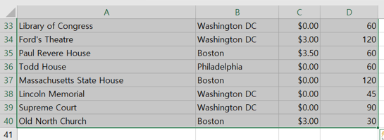
13	On the Places worksheet, sort the data by City in alphabetical order and then within City, sort by Sightseeing Locations in alphabetical order.
14	On the Places worksheet, add a total row to display the average of the Time Needed column. Apply Number format with zero decimal places to the total.
15	On the Places worksheet, select the values in the Time Needed column and apply conditional formatting to highlight cells containing values greater than 60 with Green Fill with Dark Green Text.
16	On the Places worksheet, apply a filter to display only fees that are less than or equal to $10.
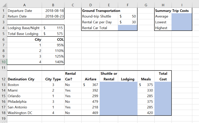
17	On the Cities worksheet, click cell F4 and enter a formula that will subtract the Departure Date (B1) from the Return Date (B2) and then multiply the result by the Rental Car per Day value (F3).
18	On the Cities worksheet, click cell E13. Depending on the city, you will either take a shuttle to/from the airport or rent a car. Insert an IF function that compares to see if Yes or No is located in the Rental Car? Column for a city. If the city contains No, display the value in cell F2. If the city contains Yes, display the value in the Rental Car Total (F4). Copy the function from cell E13 and use the Paste Formulas option to copy the function to the range E14:E18 without removing the border in cell E18.
19	On the Cities worksheet, click cell F13. The lodging is based on a multiplier by City Type. Some cities are more expensive than others. Insert a VLOOKUP function that looks up the City Type (B13), compares it to the City/COL range (A7:B10), and returns the COL percentage. Then multiply the result of the lookup function by the Total Base Lodging (B5) to get the estimated lodging for the first city. Copy the function from cell F13 and use the Paste Formulas option to copy the function to the range F14:F18 without removing the border in cell F18.
20	On the Cities worksheet, click cell H13 and enter the function that calculates the total costs for the first city. Copy the function in cell H13 and use the Paste Formulas option to copy the function to the range H14:H18 without removing the border in cell H18.
21	On the Cities worksheet, select the range E14:H18 and apply Comma Style with zero decimal places. Select the range E13:H13 and apply Accounting Number format with zero decimal places.
22	On the Cities worksheet, in cell I2, enter a function that will calculate the average total cost per city. In cell I3, enter a function that will identify the lowest total cost. In cell I4 enter a function that will return the highest total cost.
23	On the Cities worksheet, select Landscape orientation, set a 1-inch top margin, and center the worksheet data horizontally on the page.
24	Ensure that the worksheets are correctly named and placed in the following order in the workbook: DC, Places, Cities. Save the workbook. Close the workbook and then exit Excel. Submit the workbook as directed.

dc

place

cities

A B C D E F G 1 Washington DC Memorial Visitors 2 Source: https://ima.nps.gov/Stats/Reports/Park/FRDE 3 4 Year Comple 2000 2005 2010 2015 Trend 5 Lincoln Memorial 1922 4,009,145 3,638,806 6,042,315 7,941,771 6 World War II Memorial 2004 4,410,379 3,964,351 5,068,224 7 Vietnam Veterans Memo 1982 3,782,445 3,799,968 4,555,371 5,597,077 8 Korean War Veterans Me 1994 2,923,716 3,214,467 3,072,716 4,077,835 9 Franklin Delano Roosevel 1997 2,918,846 2,852,565 2,238,052 3,290,080 10 Jefferson Memorial 1943 3,458,956 2,944,976 2,436,110 1,698,656 D 60 120 60 33 Library of Congress 34 Ford's Theatre 35 Paul Revere House 36 Todd House 37 Massachusetts State House 38 Lincoln Memorial 39 Supreme Court 40 Old North Church B Washington DC Washington DC Boston Philadelphia Boston Washington DC Washington DC Boston $0.00 $3.00 $3.50 $0.00 $0.00 $0.00 $0.00 $3.00 60 120 45 90 30 41 C F G H D Ground Transportation Round-trip Shuttle $ Rental Car per Day $ Rental Car Total 50 Summary Trip Costs Average Lowest Highest 30 A B 1 Departure Date 2018-08-18 2 Return Date 2018-08-23 3 4 Lodging Base/Night $ 115 5 Total Base Lodging $ 575 6 COL 7 95% 8 2 110% 9 3 125% 10 4 140% City 1 11 Total Cost Lodging Meals $ 375 Rental City Type Car? 3 No 2 Yes Yes 3 No Yes 4 No Shuttle or Airfare Rental $367 392 299 479 218 12 Destination City 13 Boston 14 Miami 15 Orlando 16 Philadelphia 17 San Antonio 18 Washington DC 19 330 1 285 375 285 1 469 420