135 97890123456789012345678235880 A B C D E F G H I J L Take each value in column C and multiply it by its adjacent growth rate in column B (which is 1 plus the percentage expected growth) Growth Rate ABSOLUTE CELL REFERENCES Year 5 Year 2 Year 3 Year 4 Year 6 Year 7 Year 8 Year 9 (Expected) Year 0 Year 1 4 $2,500 13 Investment A N A P N A N A N A N A N A F N A N A N A 15 Formulas 17 Start in column D, then move across allowing the column to change, and multiply the preceding value by its FIXED growth rate in cell $B$13 (which is 1 plus the percentage expected growth) to get the current value FIXED COLUMN RELATIVE ROW CELL REFERENCES Growth Rate (Expected) Year 0 Year 1 4 $2,500 Year 2 Year 3 Year 4 Year 5 Year 6 Year 7 Year 8 Year 9 Investment A Investment B 11 $2,500 Investment C 8 $2,500 N A 26 Formulas N A N A N A N A N A N A N A N A N A N A N A N A N A N A N A N A N A N A N A N A N A N A N A N A N A N A 30 Start in column D, then move across, and multiply the preceding value by its growth rate in cell SB22 (which is 1 plus the percentage expected growth) to get the current value 31 By changing the growth rate cell from $B$22, etc to $B22, the row of the growth rate is allowed to change yet remain in column B while filling down to the other two Investments Sheet1 Calculation Mode Automatic Workbook Statirtier 22 23 24 fx J M Year 10 N A Year 10 N A N A N A Glus Foodback to Microsoft V 2 0 Excel Activity 2 Fixed and Relative References (Tutorial) x Question 1 0 10 Video Submit Introduction A Microsoft Excel spreadsheet is laid out in a grid of columns and rows The columns are labeled with letters A, B, C while rows are labeled with numbers 1,2,3 and so on A cell is where a column and row intersect For example, where column B intersects with row 4, the cell is labeled B4 You can think of a cell as an address on a map The data has been collected in the Microsoft Excel Online file below Open the spreadsheet and perform the required analysis to answer the questions below Open spreadsheet Relative Cell References One of the most powerful features in Excel is the ability to place a formula in one cell and then drag the contents of that cell down or across to repeat that same formula on other values For example, let's say you have this following simple layout in Excel A B D E 1 Item Order Quantity Unit Cost ($) Total Cost 11 99 2 MP3 album 8 3 Concert t shirt 17 27 99 4 Large soft drink 11 4 99 We can tell from this table that there are 8 orders for the MP3 album and that value is in cell C2 A B C D E 1 Item Order Quantity 8 Unit Cost ($) Total Cost 11 99 2 MP3 album 3 Concert t shirt 17 27 99 Autosaved at 4 37 PM Back Next 2 0 Excel Activity 2 Fixed and Relative References (Tutorial) x Question 1 0 10 4 Large soft drink 11 4 99 Submit Next, we would like to calculate the Total Cost for all MP3 orders To do that we would multiply the Order Quantity by the Unit Cost 8 11 99 That can be done in cell E2 A B D E 1 Item Order Quantity Unit Cost ($) Total Cost 11 99 2 MP3 album 8 C2 D2 3 Concert t shirt 17 27 99 4 Large soft drink 11 4 99 Finally, we can select cell E2, grab the drag handle, and then drag down to E4 to obtain the other two Total Cost values This technique uses relative cell references, meaning the values can change as you drag downward A B E D Unit Cost ($) 1 Item Total Cost Order Quantity 8 17 2 MP3 album 11 99 C2 D2 3 Concert t shirt C3 D3 27 99 4 99 4 Large soft drink 11 C4 D4 In the given spreadsheet, three investments are listed in rows 4 6 Column B contains the expected growth rate for each investment as a percentage Calculate the expected value of Investment A in cell D4 by multiplying its value in Year 0 by the quantity (1 Growth rate) Then drag cell D4 down to D6 to get the other two investment values after one year given different growth rates and place those values below Investment A $ (to the nearest dollar) Investment B $ (to the nearest dollar) Investment C $ (to the nearest dollar) Absolute Cell References Autosaved at 4 37 PM Back Next By placing a dollar sign ($) in front of the row and or column of a cell you can lock down either the row, column, or both so no change occurs when you drag to fill other cells In row 13, we would like to calculate the value of Investment A over a period of ten years assuming the constant growth rate in cell B13 First, calculate the value in Year 1 (D13) using the same technique in Part A If you try to drag D13 to the right to fill in the remaining years, you will get some very strange numbers That is because the growth rate cell B13 is changing as you drag However, you need that cell to say fixed in place for all the formulas as you drag to fill E13 through M13 The way to fix cell B13 in place is using an absolute cell reference Instead of B13 in the formula change it to $B$13 and then drag to the right to fill Year 2 through Year 10 Enter those values below (to the nearest dollar) Do not use a dollar sign ($), just the value Year 5 Year 9 Year 1 Year 2 Year 3 $ $ $ Year 4 $ 2188 Year 6 Year 7 Year 8 $ $ $ Year 10 $ $ Fixed Column Relative Row Cell References Now you would like to track the value of all three investments over the same 10 year period in rows 22, 23, and 24 Start by creating a formula in D22 that is like the formula in D13 However, there is one change to make Knowing that you will want to drag the entire 10 year span in row 22 down to rows 23 and 24, the row reference in the (1 growth rate) calculation must be able to change as you drag That is done by removing the dollar sign ($) in front of the row number in the growth calculation Make sure that i done in cell D22, then drag across to M22 to obtain the values for Investment A Finally, select all cells from D22 to M22, and then drag down to fill the next two rows Now you have the values for Investment B and Investment C Notice the format of the formulas in cells D22 M24 What is the value of each investment in year 10 Investment A $ (to the nearest dollar) Investment B $ (to the nearest dollar) Investment C $ (to the nearest dollar) Autosaved at 4 37 PM Back Next 2 0 Excel Activity 2 Fixed and Relative References (Tutorial) Question 1 0 10 Submit

Question

135 97890123456789012345678235880 A B C D E F G H I J L  Take each value in column C and multiply it by its adjacent growth rate in column B (which is 1 plus the percentage expected growth)   Growth Rate ABSOLUTE CELL REFERENCES Year 5 Year 2 Year 3 Year 4 Year 6 Year 7 Year 8 Year 9 (Expected) Year 0 Year 1 4  $2,500 13 Investment A  N A P  N A  N A  N A  N A  N A F  N A  N A  N A 15 Formulas 17  Start in column D, then move across allowing the column to change, and multiply the preceding value by its FIXED growth rate in cell $B$13 (which is 1 plus the percentage expected growth) to get the current value   FIXED COLUMN   RELATIVE ROW CELL REFERENCES Growth Rate (Expected) Year 0 Year 1 4  $2,500 Year 2 Year 3 Year 4 Year 5 Year 6 Year 7 Year 8 Year 9 Investment A Investment B 11  $2,500 Investment C 8  $2,500  N A 26 Formulas  N A  N A  N A  N A  N A  N A  N A  N A  N A  N A  N A  N A  N A  N A  N A  N A  N A  N A  N A  N A  N A  N A  N A  N A  N A  N A 30  Start in column D, then move across, and multiply the preceding value by its growth rate in cell SB22 (which is 1 plus the percentage expected growth) to get the current value   31  By changing the growth rate cell from $B$22, etc  to $B22, the row of the growth rate is allowed to change yet remain in column B while filling down to the other two Investments   Sheet1   Calculation Mode  Automatic Workbook Statirtier 22 23 24 fx J M Year 10  N A Year 10  N A  N A  N A Glus Foodback to Microsoft V 2 0 Excel Activity 2   Fixed and Relative References (Tutorial) x Question 1 0 10 Video Submit Introduction A Microsoft Excel spreadsheet is laid out in a grid of columns and rows  The columns are labeled with letters  A, B, C    while rows are labeled with numbers  1,2,3    and so on  A cell is where a column and row intersect  For example, where column B intersects with row 4, the cell is labeled B4  You can think of a cell as an address on a map  The data has been collected in the Microsoft Excel Online file below  Open the spreadsheet and perform the required analysis to answer the questions below  Open spreadsheet Relative Cell References One of the most powerful features in Excel is the ability to place a formula in one cell and then drag the contents of that cell down or across to repeat that same formula on other values  For example, let's say you have this following simple layout in Excel  A B D E 1 Item Order Quantity Unit Cost ($) Total Cost 11 99 2 MP3 album 8   3 Concert t shirt 17 27 99   4 Large soft drink 11 4 99   We can tell from this table that there are 8 orders for the MP3 album and that value is in cell C2  A B C D E 1 Item Order Quantity 8 Unit Cost ($) Total Cost 11 99 2 MP3 album   3 Concert t shirt 17 27 99   Autosaved at 4 37 PM Back Next 2 0 Excel Activity 2   Fixed and Relative References (Tutorial) x Question 1 0 10 4 Large soft drink 11 4 99   Submit Next, we would like to calculate the Total Cost for all MP3 orders  To do that we would multiply the Order Quantity by the Unit Cost  8   11 99  That can be done in cell E2  A B D E 1 Item Order Quantity Unit Cost ($) Total Cost 11 99 2 MP3 album 8  C2 D2   3 Concert t shirt 17 27 99 4 Large soft drink 11 4 99   Finally, we can select cell E2, grab the drag handle, and then drag down to E4 to obtain the other two Total Cost values  This technique uses relative cell references, meaning the values can change as you drag downward  A B E D Unit Cost ($) 1 Item Total Cost Order Quantity 8 17 2 MP3 album 11 99  C2 D2 3 Concert t shirt  C3 D3 27 99 4 99 4 Large soft drink 11  C4 D4 In the given spreadsheet, three investments are listed in rows 4 6  Column B contains the expected growth rate for each investment as a percentage  Calculate the expected value of Investment A in cell D4 by multiplying its value in Year 0 by the quantity (1   Growth rate)  Then drag cell D4 down to D6 to get the other two investment values after one year given different growth rates and place those values below  Investment A  $ (to the nearest dollar) Investment B  $ (to the nearest dollar) Investment C  $ (to the nearest dollar) Absolute Cell References Autosaved at 4 37 PM Back Next By placing a dollar sign ($) in front of the row and or column of a cell you can  lock down  either the row, column, or both so no change occurs when you drag to fill other cells  In row 13, we would like to calculate the value of Investment A over a period of ten years assuming the constant growth rate in cell B13  First, calculate the value in Year 1 (D13) using the same technique in Part A  If you try to drag D13 to the right to fill in the remaining years, you will get some very strange numbers  That is because the growth rate cell B13 is changing as you drag  However, you need that cell to say fixed in place for all the formulas as you drag to fill E13 through M13  The way to fix cell B13 in place is using an absolute cell reference  Instead of B13 in the formula change it to $B$13 and then drag to the right to fill Year 2 through Year 10  Enter those values below (to the nearest dollar)  Do not use a dollar sign ($), just the value  Year 5 Year 9 Year 1 Year 2 Year 3 $ $ $ Year 4 $ 2188 Year 6 Year 7 Year 8 $ $ $ Year 10 $ $ Fixed Column   Relative Row Cell References Now you would like to track the value of all three investments over the same 10 year period in rows 22, 23, and 24  Start by creating a formula in D22 that is like the formula in D13  However, there is one change to make  Knowing that you will want to drag the entire 10 year span in row 22 down to rows 23 and 24, the row reference in the (1   growth rate) calculation must be able to change as you drag  That is done by removing the dollar sign ($) in front of the row number in the growth calculation  Make sure that i done in cell D22, then drag across to M22 to obtain the values for Investment A  Finally, select all cells from D22 to M22, and then drag down to fill the next two rows  Now you have the values for Investment B and Investment C  Notice the format of the formulas in cells D22 M24  What is the value of each investment in year 10  Investment A  $ (to the nearest dollar) Investment B  $ (to the nearest dollar) Investment C  $ (to the nearest dollar) Autosaved at 4 37 PM Back Next 2 0 Excel Activity 2   Fixed and Relative References (Tutorial) Question 1 0 10 Submit

Accepted Answer

The Answer is in the image, click to view ...

Question

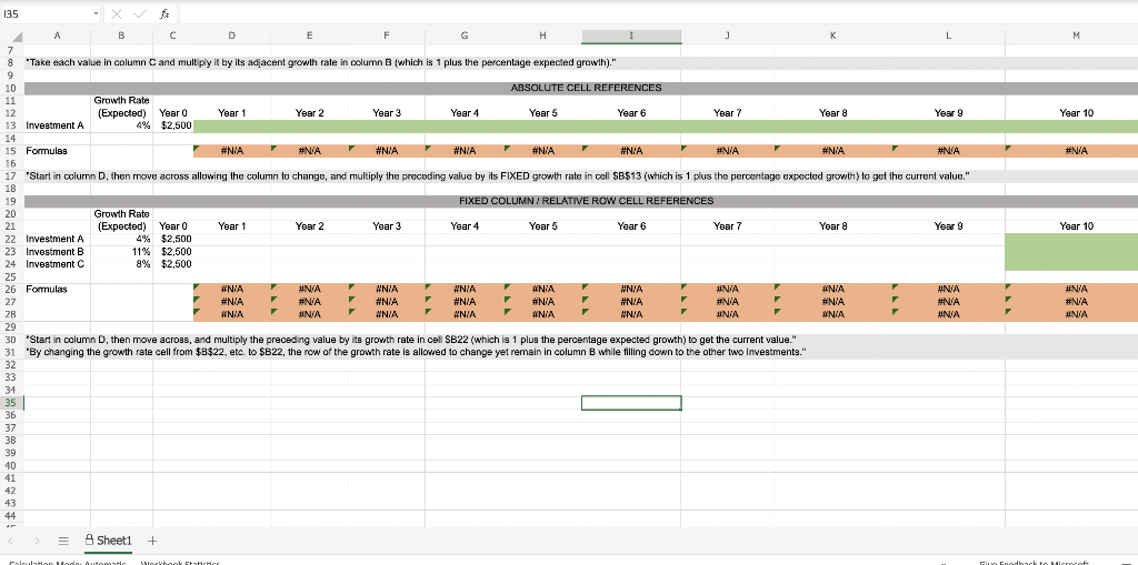
135 97890123456789012345678235880 A B C D E F G H I J L *Take each value in column C and multiply it by its adjacent

Step by Step Solution

Step: 1

Get Instant Access to Expert-Tailored Solutions

Step: 2

Step: 3

Ace Your Homework with AI

Recommended Textbook for

Risk Management In Forex How To Minimize Losses And Maximize Returns