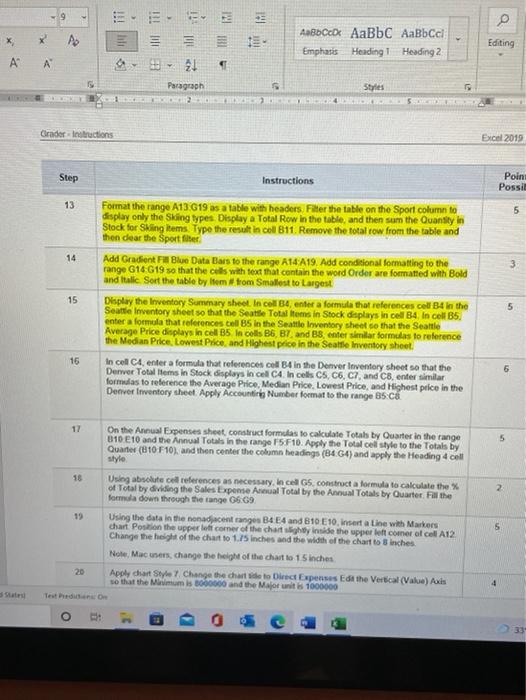
#16

X l Emphasis Heading Heading 2 Editing A A 21 Paragraph Stres 20 Crader Instructions Excel 2019 Step Instructions Point Possil 13 14 15 Format the range A13 G19 as a table with headers Filter the table on the Sport column to display only the Sking types Display a Total Row in the table, and then sum the Quantity in Stock for Sking items Type the result in col 811 Remove the total row from the table and then dear the Sportfilter Add Gradient Fan Blue Data Bars to the range A1:A19. Add conditional formatting to the range G14 G19 so that the cells with text that contain the word Order are formatted with Bold and Italic Sort the table by Item from Smallest to Largest Display the Inventory Summary sheet. In cell 84, enter a formula that references cell B4 in the Seattle Inventory sheet so that the Seattle Total Items in Stock displays in cell B4. In cell B5. enter a formula that references cells in the Seattle Inventory sheet so that the Seattle Average Price dinplays in cell B5 In colls B6 B7 and 38 enter similar formulas to reference the Media Price, Lowest Price and Highest price in the Seattle Inventory sheet in cell CA, enter a formula that references coll B4 in the Denver Inventory sheet so that the Derwer Total Items in Stock displays in cel C4. In cells C5, C6, C7, and Center similar formulas to reference the average Price, Median Price, Lowest Price, and Highest price in the Denver Inventory sheet Apply Accounting Number format to the range 85.co 5 15 6 17 On the Annual Expenses sheet construct formulas to calculate Totals by Quarter in the range 010 E10 and the Annual Totals in the range 15 F10. Apply the Total cell style to the Totals by Quarter (810 F10), and then center the column headings (84.G4) and apply the Heading 4 cell style 18 2 19 Using absolute coreferences as necessary. In cell GS. construct a formula to calculate the of Total by dividing the Sales Expense Anual Total by the Annual Totals by Quarter Fall the forma down through the tange 06.09 Using the data in the nonadjacent ranges B4 E4 and 810 E10, Insert a Line with Markers chart Position the upper left comer of the chartslightly Inside the upper left corner of cel A12 Change the height of the chart to 1.75 inches and the width of the chart to inches Note, Mac users, change the height of the chart to 15 inches Apply chart Style 1 Change the chartside to Direct Expenses Edit the Vertical (Value) Axis so that the Minum is 1000000 and the Major unit is 1000000 5 20 4 Test the O 3 X l Emphasis Heading Heading 2 Editing A A 21 Paragraph Stres 20 Crader Instructions Excel 2019 Step Instructions Point Possil 13 14 15 Format the range A13 G19 as a table with headers Filter the table on the Sport column to display only the Sking types Display a Total Row in the table, and then sum the Quantity in Stock for Sking items Type the result in col 811 Remove the total row from the table and then dear the Sportfilter Add Gradient Fan Blue Data Bars to the range A1:A19. Add conditional formatting to the range G14 G19 so that the cells with text that contain the word Order are formatted with Bold and Italic Sort the table by Item from Smallest to Largest Display the Inventory Summary sheet. In cell 84, enter a formula that references cell B4 in the Seattle Inventory sheet so that the Seattle Total Items in Stock displays in cell B4. In cell B5. enter a formula that references cells in the Seattle Inventory sheet so that the Seattle Average Price dinplays in cell B5 In colls B6 B7 and 38 enter similar formulas to reference the Media Price, Lowest Price and Highest price in the Seattle Inventory sheet in cell CA, enter a formula that references coll B4 in the Denver Inventory sheet so that the Derwer Total Items in Stock displays in cel C4. In cells C5, C6, C7, and Center similar formulas to reference the average Price, Median Price, Lowest Price, and Highest price in the Denver Inventory sheet Apply Accounting Number format to the range 85.co 5 15 6 17 On the Annual Expenses sheet construct formulas to calculate Totals by Quarter in the range 010 E10 and the Annual Totals in the range 15 F10. Apply the Total cell style to the Totals by Quarter (810 F10), and then center the column headings (84.G4) and apply the Heading 4 cell style 18 2 19 Using absolute coreferences as necessary. In cell GS. construct a formula to calculate the of Total by dividing the Sales Expense Anual Total by the Annual Totals by Quarter Fall the forma down through the tange 06.09 Using the data in the nonadjacent ranges B4 E4 and 810 E10, Insert a Line with Markers chart Position the upper left comer of the chartslightly Inside the upper left corner of cel A12 Change the height of the chart to 1.75 inches and the width of the chart to inches Note, Mac users, change the height of the chart to 15 inches Apply chart Style 1 Change the chartside to Direct Expenses Edit the Vertical (Value) Axis so that the Minum is 1000000 and the Major unit is 1000000 5 20 4 Test the O 3