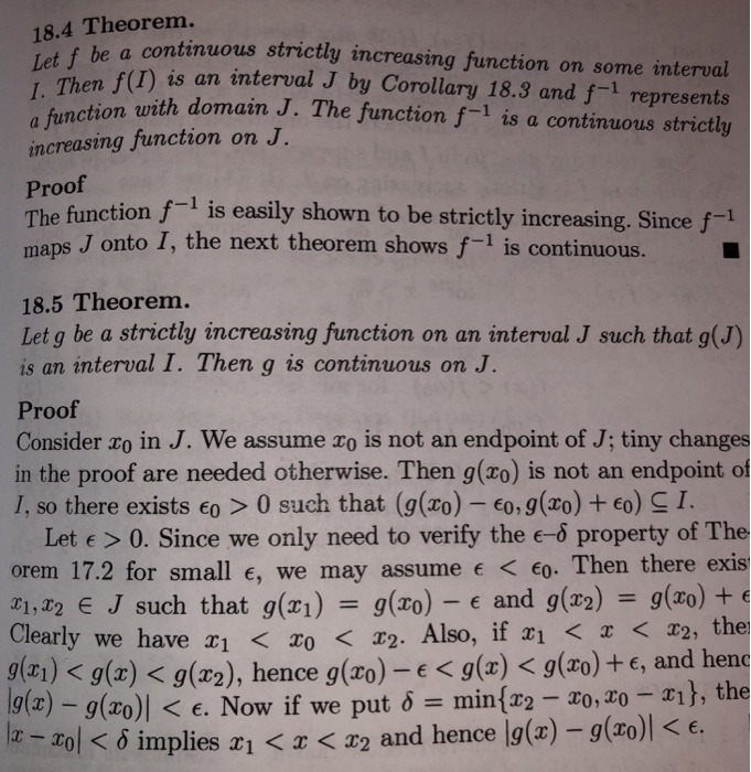
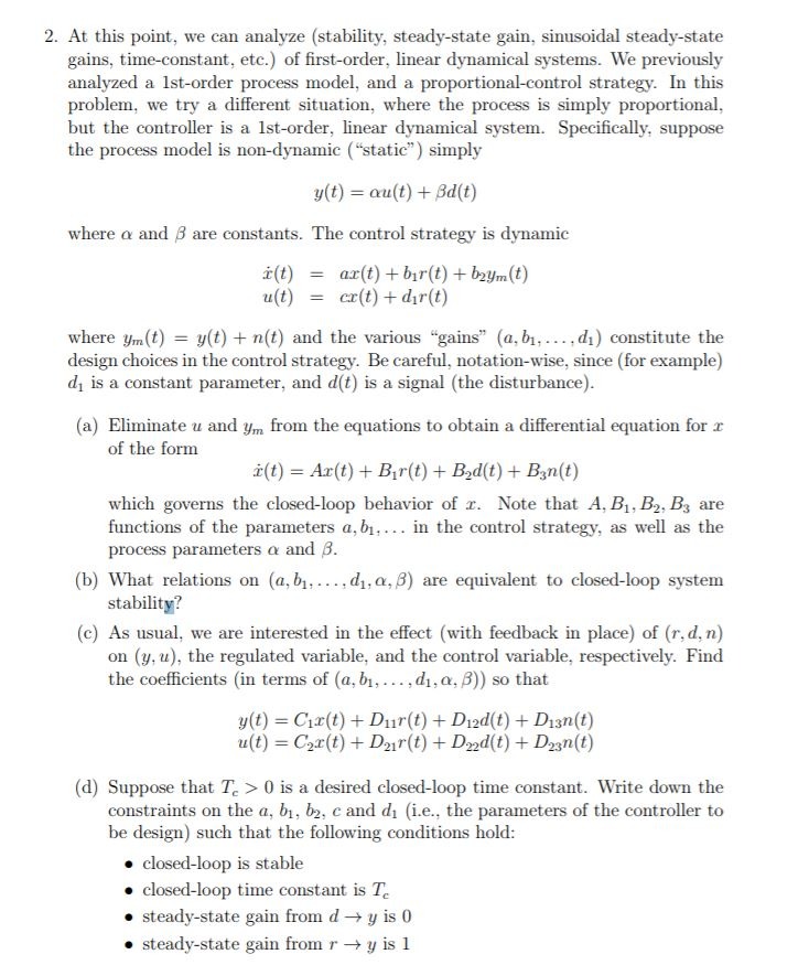
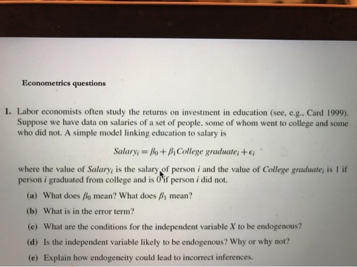
18.4 Theorem. Let f be a continuous strictly increasing function on some interval 1. Then f(1) is an interval J by Corollary 18.3 and f-1 represents a function with domain J. The function f-1 is a continuous strictly increasing function on J. Proof The function fis easily shown to be strictly increasing. Since f maps J onto I, the next theorem shows f-1 is continuous. 18.5 Theorem. Let g be a strictly increasing function on an interval J such that g(J) is an interval I. Then g is continuous on J. Proof Consider co in J. We assume To is not an endpoint of J; tiny changes in the proof are needed otherwise. Then g(x0) is not an endpoint of I, so there exists co > 0 such that (g(To) - co, g(x0) + co) CI. Let 0. Since we only need to verify the e-o property of The orem 17.2 for small e, we may assume e 0 is a desired closed-loop time constant. Write down the constraints on the a, b1, b2, c and di (i.e., the parameters of the controller to be design) such that the following conditions hold: . closed-loop is stable . closed-loop time constant is To . steady-state gain from d -> y is 0 . steady-state gain from r - y is 12. At this point, we can analyze (stability, steady-state gain, sinusoidal steady-state gains, time-constant, etc.) of first-order, linear dynamical systems. We previously analyzed a Ist-order process model, and a proportional-control strategy. In this problem, we try a different situation, where the process is simply proportional, but the controller is a Ist-order, linear dynamical system. Specifically, suppose the process model is non-dynamic ("static" ) simply y(t) = cu(t) + Bd(t) where o and B are constants. The control strategy is dynamic i (t) = ar(t) + bir(t) + bzym(t) u(t) = cr(t) + dir(t) where ym(t) = y(t) + n(t) and the various "gains" (a, bi, . .., di) constitute the design choices in the control strategy. Be careful, notation-wise, since (for example) d, is a constant parameter, and d(t) is a signal (the disturbance). (a) Eliminate u and ym from the equations to obtain a differential equation for r of the form r(t) = Ar(t) + Bir(t) + Bad(t) + Ban(t) which governs the closed-loop behavior of r. Note that A, B1, B2, By are functions of the parameters a, b1, ... in the control strategy, as well as the process parameters o and B. (b) What relations on (a, b1. .... dj, or, B) are equivalent to closed-loop system stability? (c) As usual, we are interested in the effect (with feedback in place) of (r, d, n) on (y, u), the regulated variable, and the control variable, respectively. Find the coefficients (in terms of (a, bi, . . ., d1, 0, B)) so that y(t) = Cix(t) + Dur(t) + Died(t) + Dian(t) u(t) = Car(t) + Dar(t) + Dad(t) + Dzan(t) (d) Suppose that T. > 0 is a desired closed-loop time constant. Write down the constraints on the a, b1, b2, c and di (i.e., the parameters of the controller to be design) such that the following conditions hold: . closed-loop is stable . closed-loop time constant is To . steady-state gain from d -> y is 0 . steady-state gain from r - y is 1Econometrics questions 1. Labor economists often study the returns on investment in education (see, e.g., Card 1999). Suppose we have data on salaries of a set of people. some of whom went to college and some who did not. A simple model linking education to salary is Salary, = Bo + By College graduate, + er where the value of Salary, is the salary of person i and the value of College graduate; is 1 if person i graduated from college and is O' if person i did not. (a) What does Bo mean? What does , mean? (b) What is in the error term? (c) What are the conditions for the independent variable X to be endogenous? (d) Is the independent variable likely to be endogenous? Why or why not? (e) Explain how endogeneity could lead to incorrect inferences


