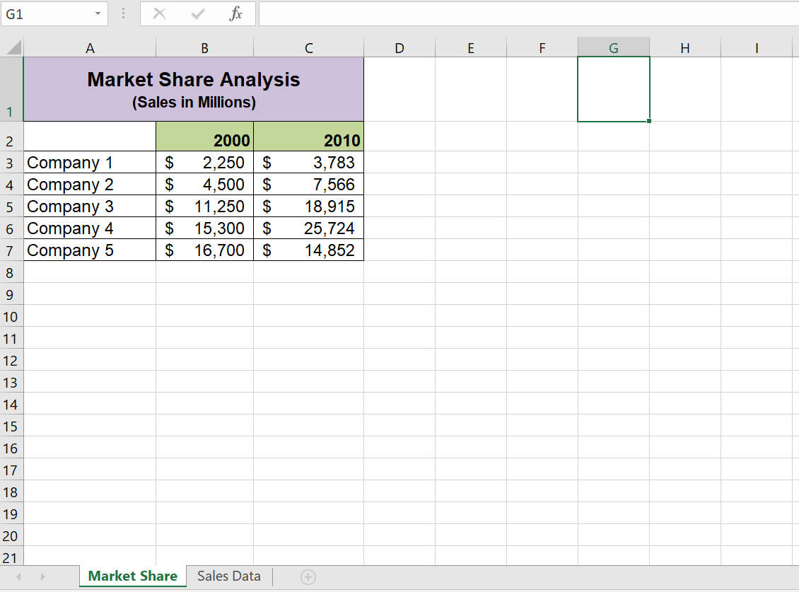
1.Create a pie chart using the data in the Market Share worksheet. The pie chart should show the percent of total for only the year 2000. Use the Exploded Pie in 3-D format.

2. Move the chart so the upper left corner is in the center of cell E2. 3. Resize the chart so the left side is locked to the left side of Column E, the right side is locked to the right side of Column M, the top is locked to the top of Row 2, and the bottom is locked to the bottom of Row 17.

4. Remove the legend.

5. Change the chart title to the following: Market Share for the Year 2000.

6. Add the Category Name and Percentage data labels to the outside end of each section of the pie chart.

7. Bold the data labels and change the font style to Arial.

8. Create a 100% stacked column chart using the data in the Market Shareworksheet. The stacked column chart should show the percentages 0% to 100% along the Y axis. The X axis should show stacks for the year 2000 and 2010. There should only be two stacks, or columns, in the plot area showing the percent of total for each company.

9. Move the 100% stacked column chart to a separate chart sheet. The tab name for the chart sheet should read Market Share Chart.

10. Remove the legend on the stacked column chart and add a data table with legend keys below the X axis.

11. Add a title above the chart that reads 10-Year Change in Market Share.

12. Format the chart title using the Subtle Effect - Red, Accent 2 preset shape style. Change the font style to Arial and the font size to 20 points.

13. Add a Y axis title that reads Market Share. Use the Rotated Title alignment.

14. Format the Y axis title using the Subtle Effect - Red, Accent 2 preset shape style. Change the font style to Arial and the font size to 16 points.

15. Format the X and Y axes by changing the font style to Arial, making the font bold, and changing the font size to 14 points.

16. Change the fill color of the chart area to Tan, Background 2, Darker 10%.

17. Add series lines that connect each section of the two stacks in the plot area.

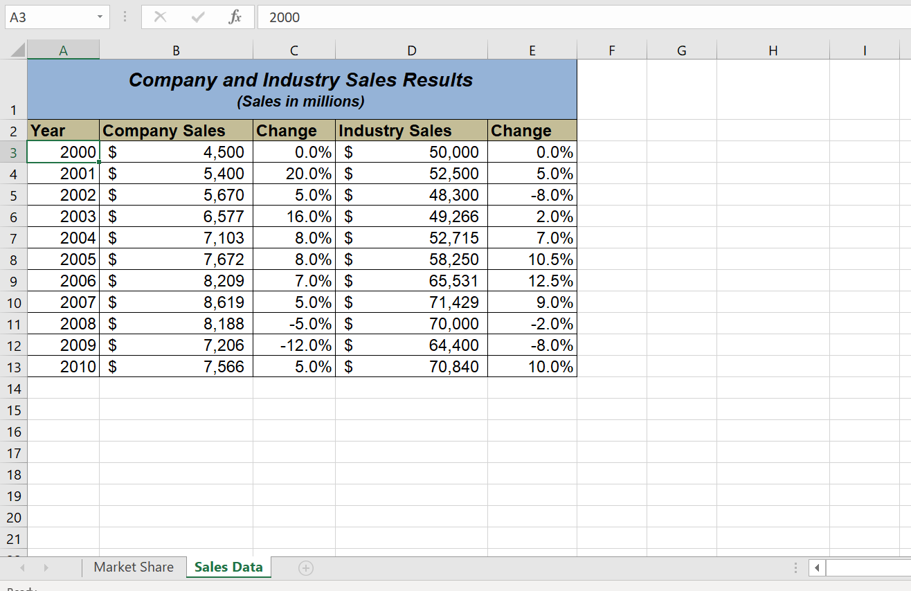
18. Create a column chart showing just the Company Sales in the Sales Dataworksheet. The chart should show the Company Sales in the range B3:B13 along the Y axis. The years in the range A3:A13 should appear on the X axis. Use the basic 2-D Clustered Column format. The series name should be Gross Sales.

19. Move the column chart to a separate chart sheet. The tab name for the chart sheet should read Company Sales Chart. Remove the legend on the column chart. Then format the X and Y axes by changing the font style to Arial, making the font bold, and changing the font size to 16 points.

21. Reduce the height of the plot area by approximately one inch. There should be about one inch of space between the bottom of the chart title and the top of the plot area.

22. Add an annotation above the Y axis that reads Sales in Millions. Format the annotation with an Arial font style, bold font, italics font, and font size of 14 points. 23. Change the color of the bars in the plot area to dark red.

24. Create a line chart comparing the change in sales for the company and overall industry in the Sales Data worksheet. Construct the chart as follows: o The Y axis should show the growth percentages for the company in the range C3:C13 and the growth percentages for the industry in the range E3:E13. o The series name for the company growth percentages should beCompany. o The series name for the industry growth percentages should beIndustry. o The years in the range A3:A13 should appear on the X axis. o Use the Line with Markers format.

25. Move the chart so the upper left corner is in the center of cell G2.

26. Resize the chart so the left side is locked to the left side of Column G, the right side is locked to the right side of Column P, the top is locked to the top of Row 2, and the bottom is locked to the bottom of Row 18.

27. Adjust the scale of the Y axis so the maximum value is set to .20.

28. Format the values on the Y axis so there are zero decimal places.

29. Save the workbook by adding your name in front of the current workbook name (i.e., your name Chapter 4 Skills Test). 30. Close the workbook and Excel.

G1 fo A B D E F H | Market Share Analysis (Sales in Millions) 1 2 3 Company 1 4 Company 2 5 Company 3 6 Company 4 7 Company 5 $ $ $ $ $ 2000 2,250 $ 4,500 $ 11,250 $ 15,300 $ 16,700 $ 2010 3,783 7,566 18,915 25,724 14,852 8 9 10 11 12 13 14 15 16 17 18 19 20 21 Market Share Sales Data x fic 2000 A B D E F G H Company and Industry Sales Results (Sales in millions) 1 2 Year Company Sales Change Industry Sales Change 3 2000 $ 4,500 0.0% $ 50,000 0.0% 4 2001 $ 5,400 20.0% $ 52,500 5.0% 5 2002 $ 5,670 5.0% $ 48,300 -8.0% 6 2003 $ 6,577 16.0% $ 49,266 2.0% 7 2004 $ 7,103 8.0% $ 52,715 7.0% 8 2005 $ 7,672 8.0% $ 58,250 10.5% 9 2006 $ 8,209 7.0% $ 65,531 12.5% 10 2007 $ 8,619 5.0% $ 71,429 9.0% 11 2008 $ 8,188 -5.0% $ 70,000 -2.0% 12 2009 $ 7,206 -12.0% $ 64,400 -8.0% 13 2010 $ 7,566 5.0% $ 70,840 10.0% 14 15 16 17 18 19 20 21 Market Share Sales Data G1 fo A B D E F H | Market Share Analysis (Sales in Millions) 1 2 3 Company 1 4 Company 2 5 Company 3 6 Company 4 7 Company 5 $ $ $ $ $ 2000 2,250 $ 4,500 $ 11,250 $ 15,300 $ 16,700 $ 2010 3,783 7,566 18,915 25,724 14,852 8 9 10 11 12 13 14 15 16 17 18 19 20 21 Market Share Sales Data x fic 2000 A B D E F G H Company and Industry Sales Results (Sales in millions) 1 2 Year Company Sales Change Industry Sales Change 3 2000 $ 4,500 0.0% $ 50,000 0.0% 4 2001 $ 5,400 20.0% $ 52,500 5.0% 5 2002 $ 5,670 5.0% $ 48,300 -8.0% 6 2003 $ 6,577 16.0% $ 49,266 2.0% 7 2004 $ 7,103 8.0% $ 52,715 7.0% 8 2005 $ 7,672 8.0% $ 58,250 10.5% 9 2006 $ 8,209 7.0% $ 65,531 12.5% 10 2007 $ 8,619 5.0% $ 71,429 9.0% 11 2008 $ 8,188 -5.0% $ 70,000 -2.0% 12 2009 $ 7,206 -12.0% $ 64,400 -8.0% 13 2010 $ 7,566 5.0% $ 70,840 10.0% 14 15 16 17 18 19 20 21 Market Share Sales Data