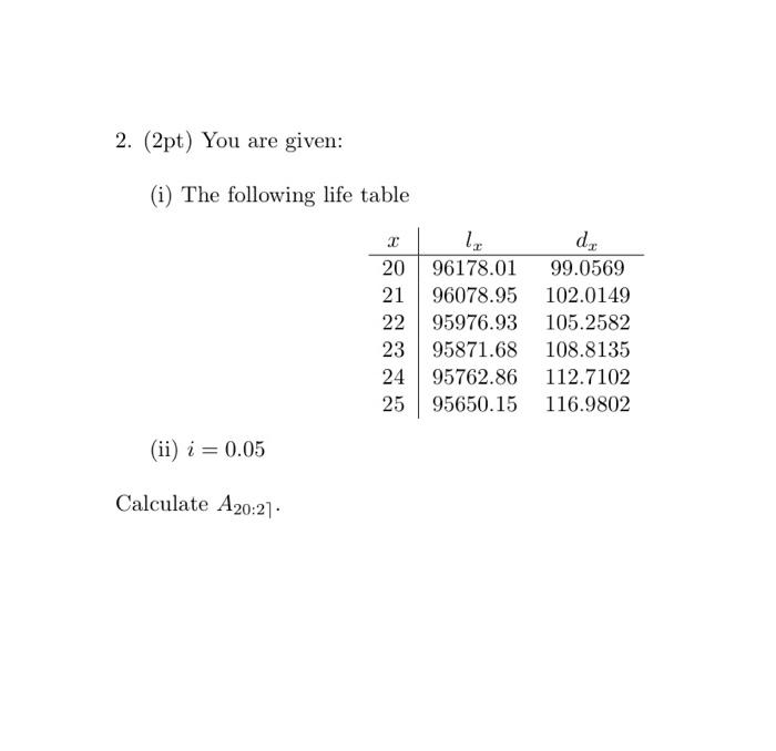
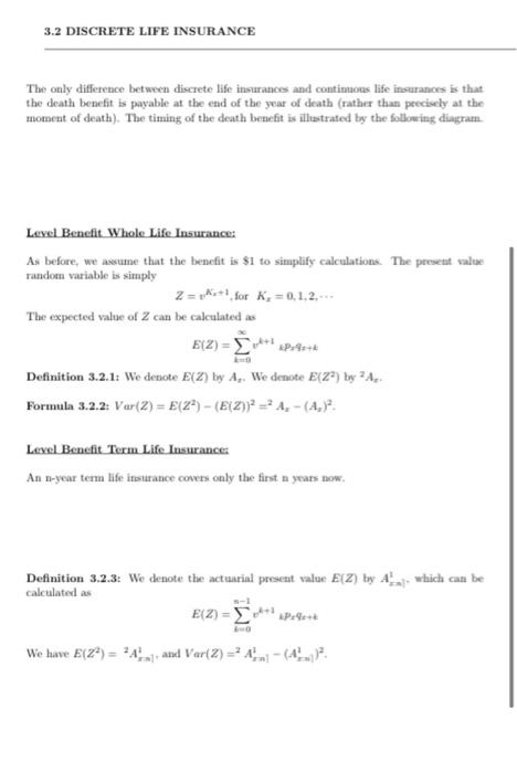
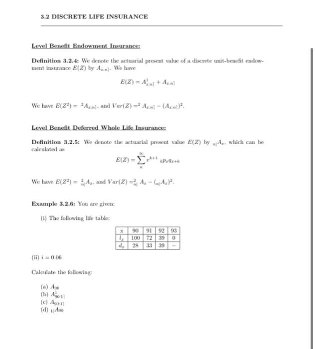
2. (2pt) You are given: (i) The following life table 20 21 22 1, 96178.01 96078.95 95976.93 95871.68 95762.86 95650.15 d. 99.0569 102.0149 105.2582 108.8135 112.7102 116.9802 23 24 25 (ii) i = 0.05 Calculate A20:21 3.2 DISCRETE LIFE INSURANCE The only difference between discrete life insurances and continuous life insurances is that the death benefit is payable at the end of the year of death (rather than precisely at the moment of death). The timing of the death benefit is illustrated by the following diagram. Level Benefit Whole Life Insurance: As before, we assume that the benefit is $1 to simplify calculations. The presett value random variable is simply Z=K+ for k, = 0,1.2.. The expected value of Z can be calculated as E(2) Definition 3.2.1: We denote E(2) by A. We denote E{Z) bwy? Formula 3.2.2: Var (2) = E(27) - (E{2)) => A, - (A,)? Level Benefit Term Life Insurancez An t-year term life insurance covers only the first years now. Definition 3.2.3: We denote the actuarial present value. E(Z) by which can be calculated as E(2) P. We have E(Z) = 24) and Var(2) = .-() 3.2 DISCRETE LIFE INSURANCE Level Benefit Endowment Insurances Definition 3.2.4: We denote the actuarial present value of a discrete unit-benefit endow- ment insurance E(Z) by Axn. We have E(Z) = A + An We have E(Z) = ?Azn and Var(2)=4,- (Au)? Level Benefit Deferred Whole Life Insurance Definition 3.2.5: We denote the actuarial present value E(Z) by 14, which can be calculated as E(2) P9z+* We have E(24) = ? Az, and Var(2)= A. - (A.)? Example 3.2.6: You are given: (1) The following life table: 90 91 9233 10072 39 0 28 dy (H) i = 0.06 Calculate the following: (a) Ano (b) 0.11 (c) Ago! (d) 490 2. (2pt) You are given: (i) The following life table 20 21 22 1, 96178.01 96078.95 95976.93 95871.68 95762.86 95650.15 d. 99.0569 102.0149 105.2582 108.8135 112.7102 116.9802 23 24 25 (ii) i = 0.05 Calculate A20:21 3.2 DISCRETE LIFE INSURANCE The only difference between discrete life insurances and continuous life insurances is that the death benefit is payable at the end of the year of death (rather than precisely at the moment of death). The timing of the death benefit is illustrated by the following diagram. Level Benefit Whole Life Insurance: As before, we assume that the benefit is $1 to simplify calculations. The presett value random variable is simply Z=K+ for k, = 0,1.2.. The expected value of Z can be calculated as E(2) Definition 3.2.1: We denote E(2) by A. We denote E{Z) bwy? Formula 3.2.2: Var (2) = E(27) - (E{2)) => A, - (A,)? Level Benefit Term Life Insurancez An t-year term life insurance covers only the first years now. Definition 3.2.3: We denote the actuarial present value. E(Z) by which can be calculated as E(2) P. We have E(Z) = 24) and Var(2) = .-() 3.2 DISCRETE LIFE INSURANCE Level Benefit Endowment Insurances Definition 3.2.4: We denote the actuarial present value of a discrete unit-benefit endow- ment insurance E(Z) by Axn. We have E(Z) = A + An We have E(Z) = ?Azn and Var(2)=4,- (Au)? Level Benefit Deferred Whole Life Insurance Definition 3.2.5: We denote the actuarial present value E(Z) by 14, which can be calculated as E(2) P9z+* We have E(24) = ? Az, and Var(2)= A. - (A.)? Example 3.2.6: You are given: (1) The following life table: 90 91 9233 10072 39 0 28 dy (H) i = 0.06 Calculate the following: (a) Ano (b) 0.11 (c) Ago! (d) 490


