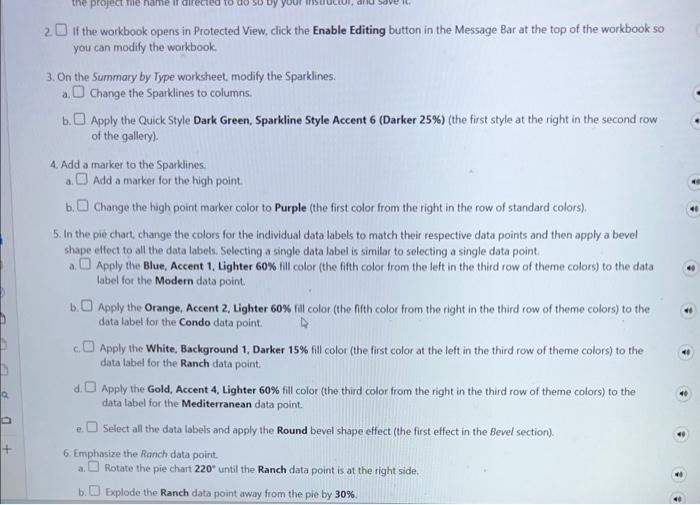
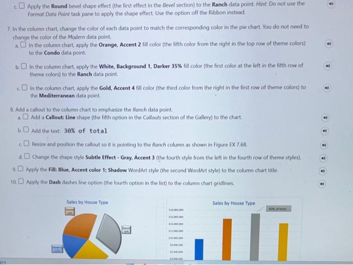
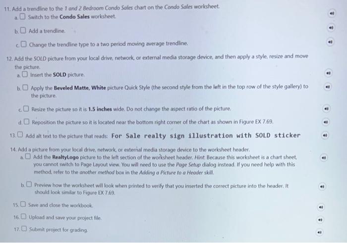
2 If the workbook opens in Protected View, click the Enable Editing button in the Message Bar at the top of the workbook so you can modify the workbook. 3. On the Summary by Type worksheet, modify the Sparklines. a. Change the Sparklines to columns. b. Apply the Quick Style Dark Green, Sparkline Style Accent 6 (Darker 25\%) (the first style at the right in the second row of the gallery). 4. Add a marker to the Sparklines. a. Add a marke for the high point. b. Change the high point marker color to Purple (the first color from the right in the row of standard colors). 5. In the pie chart, change the colors for the individual data labels to match their respective data points and then apply a bevel shape effect to all the data labels. Selecting a single data label is similar to selecting a single data point. a. Apply the Blue, Accent 1. Lighter 60% fill color (the fifth color from the left in the third row of theme colors) to the data label for the Modem data point. b Apply the Orange, Accent 2, Lighter 60\% fill color (the fifth color from the right in the third row of theme colors) to the data label for the Condo data point. c. Apply the White, Background 1, Darker 15% fill color (the first color at the left in the third row of theme colors) to the data label for the Ranch data point. d. Apply the Gold, Accent 4, Lighter 60% fill color (the third color from the right in the third row of theme colors) to the data label for the Mediterranean data point. e. Select all the data lobels and apply the Round bevel shape effect (the first effect in the Bevel section). 6. Emphasize the Ranch data point. a. Rotate the pie chart 220 until the Ranch data point is at the right side. b. Explode the Ranch data point away from the pie by 30%. Apply the Round bevel shape effect (the first effect in the Bevel section) to the Ranch data point. Hint: Do not use the Format Data Point task pane to apply the shape effect. Use the option off the Ribbon instead. 7. In the column chart, change the color of each data point to match the corresponding color in the pie chart. You do not need to change the color of the Modern data point. a In the column chart, apply the Orange, Accent 2 fill color (the fifth color from the right in the top row of theme colors) to the Condo data point. b. In the column chart, apply the White, Background 1, Darker 35\% fill color (the first color at the left in the fitth row of theme colors) to the Ranch data point. In the column chart, apply the Gold, Accent 4 fill color (the third color from the right in the first row of theme colors) to the Mediterranean data point. 8. Add a callout to the column chart to emphasize the Ronch data point. a Add a Callout: Line shape (the fifth option in the Callouts section of the Gallery) to the chart. b) Add the text: 30% of total c. Resize and position the callout so it is pointing to the Ranch column as shown in Figure EX 7.68. d Change the shape style Subtle Effect - Gray. Accent 3 (the fourth style from the left in the fourth row of theme styles). 9. Apply the Fill: Blue, Accent color 1; Shadow WordArt style (the second WordArt style) to the column chart title. 10 Apply the Dash dashes line option (the fourth option in the list) to the column chart gridlines. 11. Add a trendline to the 1 and 2 Bedroom Condo Sales chart on the Condo Soles worksheet. a Switch to the Condo Sales worksheet. b. Add a trendline. c Change the trendline type to a two period moving average trendline. 12. Add the SOLD picture from your local drive, network, or external media storage device, and then apply a style, resize and move the picture. a. Insert the SOLD picture. b. Apply the Beveled Matte, White picture Quick Style (the second style from the left in the top row of the style gallery) to the picture. Resize the picture so it is 1.5 inches wide. Do not change the aspect ratio of the picture. d Reposition the picture so it is located near the bottom right corner of the chart as shown in Figure EX 7.69. 13. Add alt text to the picture that reads: For Sale realty s1gn 11lustration with SOLD sticker 14. Add a picture from your local dive, network, or external media storage device to the worksheet header. a Add the Realtylogo picture to the left section of the worksheet header. Hint: Because this worksheet is a chart sheet, you cannot switch to Page Layout view. You will need to use the Poge Setup dialog instead. If you need help with this method. refer to the another method box in the Adding a Picture to a Header skill. b. Preview how the worksheet will look when printed to verify that you inserted the correct picture into the header, it should look similar to Figure EX 7.69. 15 Save and dose the workbook. 16. Upload and save your project file. 17. Submit project for grading. 2 If the workbook opens in Protected View, click the Enable Editing button in the Message Bar at the top of the workbook so you can modify the workbook. 3. On the Summary by Type worksheet, modify the Sparklines. a. Change the Sparklines to columns. b. Apply the Quick Style Dark Green, Sparkline Style Accent 6 (Darker 25\%) (the first style at the right in the second row of the gallery). 4. Add a marker to the Sparklines. a. Add a marke for the high point. b. Change the high point marker color to Purple (the first color from the right in the row of standard colors). 5. In the pie chart, change the colors for the individual data labels to match their respective data points and then apply a bevel shape effect to all the data labels. Selecting a single data label is similar to selecting a single data point. a. Apply the Blue, Accent 1. Lighter 60% fill color (the fifth color from the left in the third row of theme colors) to the data label for the Modem data point. b Apply the Orange, Accent 2, Lighter 60\% fill color (the fifth color from the right in the third row of theme colors) to the data label for the Condo data point. c. Apply the White, Background 1, Darker 15% fill color (the first color at the left in the third row of theme colors) to the data label for the Ranch data point. d. Apply the Gold, Accent 4, Lighter 60% fill color (the third color from the right in the third row of theme colors) to the data label for the Mediterranean data point. e. Select all the data lobels and apply the Round bevel shape effect (the first effect in the Bevel section). 6. Emphasize the Ranch data point. a. Rotate the pie chart 220 until the Ranch data point is at the right side. b. Explode the Ranch data point away from the pie by 30%. Apply the Round bevel shape effect (the first effect in the Bevel section) to the Ranch data point. Hint: Do not use the Format Data Point task pane to apply the shape effect. Use the option off the Ribbon instead. 7. In the column chart, change the color of each data point to match the corresponding color in the pie chart. You do not need to change the color of the Modern data point. a In the column chart, apply the Orange, Accent 2 fill color (the fifth color from the right in the top row of theme colors) to the Condo data point. b. In the column chart, apply the White, Background 1, Darker 35\% fill color (the first color at the left in the fitth row of theme colors) to the Ranch data point. In the column chart, apply the Gold, Accent 4 fill color (the third color from the right in the first row of theme colors) to the Mediterranean data point. 8. Add a callout to the column chart to emphasize the Ronch data point. a Add a Callout: Line shape (the fifth option in the Callouts section of the Gallery) to the chart. b) Add the text: 30% of total c. Resize and position the callout so it is pointing to the Ranch column as shown in Figure EX 7.68. d Change the shape style Subtle Effect - Gray. Accent 3 (the fourth style from the left in the fourth row of theme styles). 9. Apply the Fill: Blue, Accent color 1; Shadow WordArt style (the second WordArt style) to the column chart title. 10 Apply the Dash dashes line option (the fourth option in the list) to the column chart gridlines. 11. Add a trendline to the 1 and 2 Bedroom Condo Sales chart on the Condo Soles worksheet. a Switch to the Condo Sales worksheet. b. Add a trendline. c Change the trendline type to a two period moving average trendline. 12. Add the SOLD picture from your local drive, network, or external media storage device, and then apply a style, resize and move the picture. a. Insert the SOLD picture. b. Apply the Beveled Matte, White picture Quick Style (the second style from the left in the top row of the style gallery) to the picture. Resize the picture so it is 1.5 inches wide. Do not change the aspect ratio of the picture. d Reposition the picture so it is located near the bottom right corner of the chart as shown in Figure EX 7.69. 13. Add alt text to the picture that reads: For Sale realty s1gn 11lustration with SOLD sticker 14. Add a picture from your local dive, network, or external media storage device to the worksheet header. a Add the Realtylogo picture to the left section of the worksheet header. Hint: Because this worksheet is a chart sheet, you cannot switch to Page Layout view. You will need to use the Poge Setup dialog instead. If you need help with this method. refer to the another method box in the Adding a Picture to a Header skill. b. Preview how the worksheet will look when printed to verify that you inserted the correct picture into the header, it should look similar to Figure EX 7.69. 15 Save and dose the workbook. 16. Upload and save your project file. 17. Submit project for grading