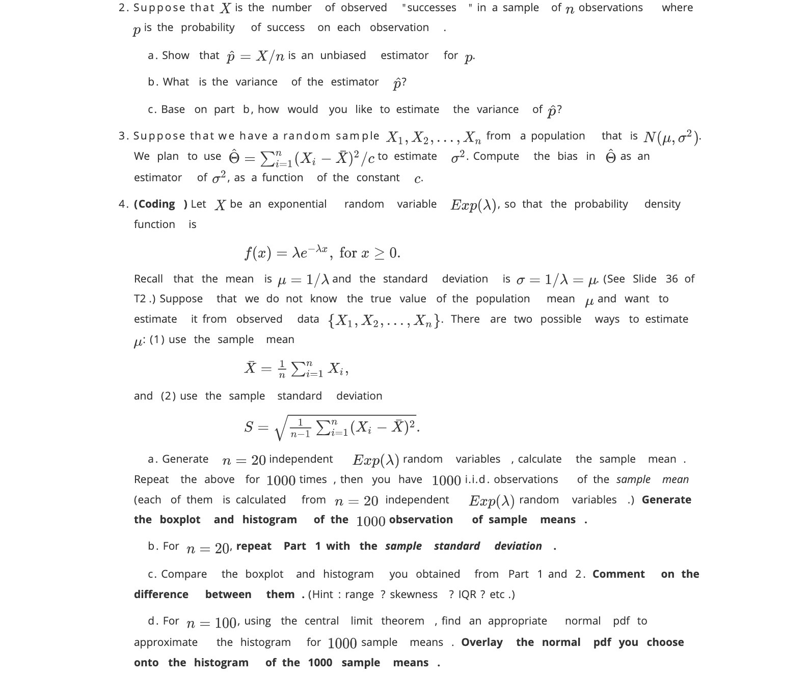
2. Suppose that X is the number of observed "successes " in a sample of n observations where p is the probability of success on each observation a. Show that p = X is an unbiased estimator for p. b. What is the variance of the estimator p? c. Base on part b, how would you like to estimate the variance of p? 3. Suppose that we have a random sample X1, X2, ..., Xn from a population that is N (u, 62 ). We plan to use ( = Liz(Xi - X) / c to estimate 2. Compute the bias in ( as an estimator of 2, as a function of the constant C. 4. (Coding ) Let X be an exponential random variable Exp()), so that the probability density function is f(x) = de-Ax, for x 2 0. Recall that the mean is u = 1/) and the standard deviation is o = 1/1 =M. (See Slide 36 of T2 .) Suppose that we do not know the true value of the population mean u and want to estimate it from observed data { X1, X2, ..., Xn). There are two possible ways to estimate M: (1) use the sample mean Li=1 Xi, and (2) use the sample standard deviation S = VnI Et(Xi - X) 2. a. Generate n = 20 independent Exp()) random variables , calculate the sample mean . Repeat the above for 1000 times , then you have 1000 i.i.d. observations of the sample mean (each of them is calculated from n = 20 independent Exp()) random variables .) Generate the boxplot and histogram of the 1000 observation of sample means . b. For n = 20, repeat Part 1 with the sample standard deviation c. Compare the boxplot and histogram you obtained from Part 1 and 2. Comment on the difference between them . (Hint : range ? skewness ? IQR ? etc.) d. For n = 100, using the central limit theorem , find an appropriate normal pdf to approximate the histogram for 1000 sample means . Overlay the normal pdf you choose onto the histogram of the 1000 sample means