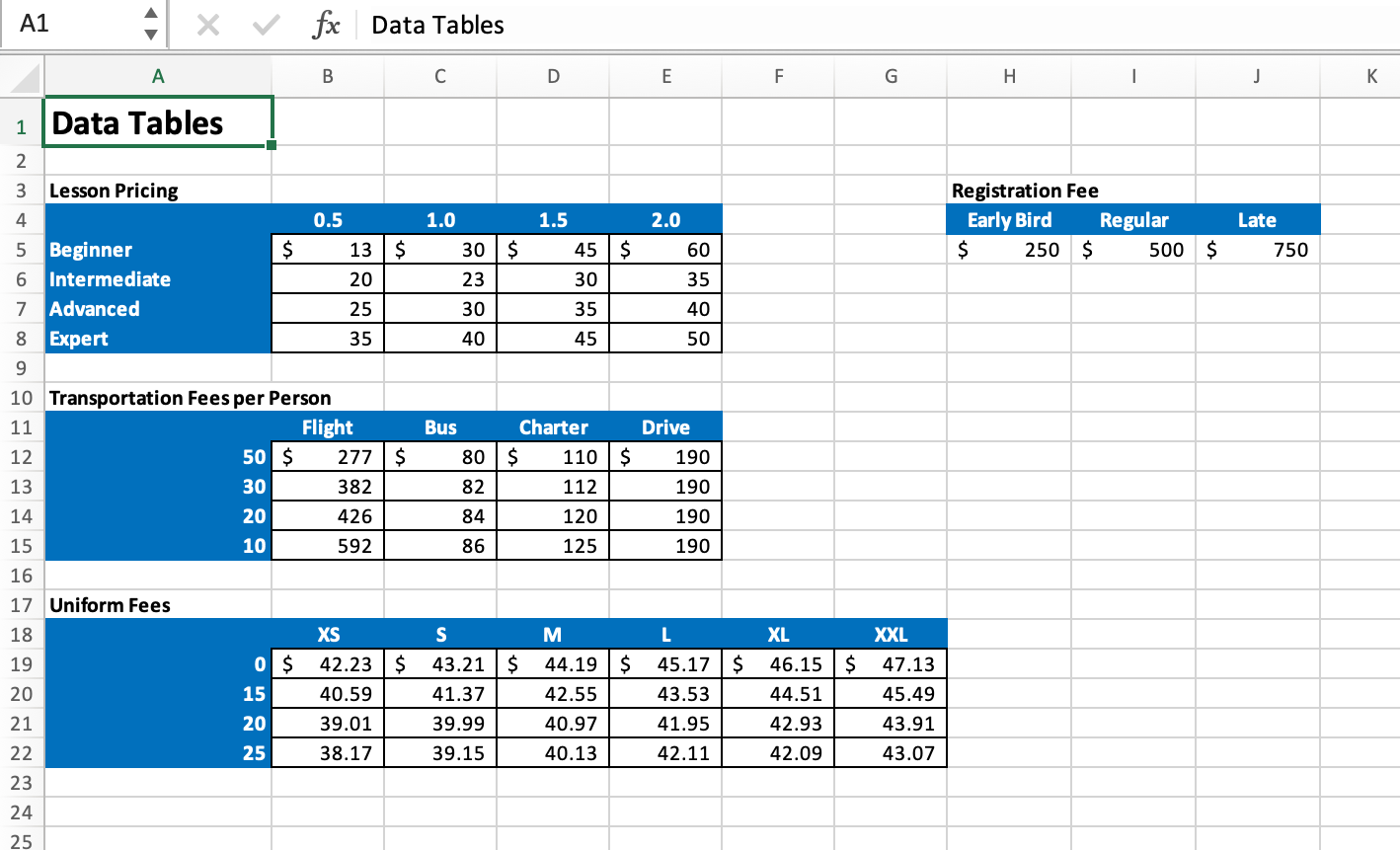
2	The DataTables worksheet contains 4 tables listing the various prices and fees that Fiddlers charges their clients. It is common practice to have all pricing tables on one worksheet. Creating named ranges for these tables will make it easier to refer to them from other worksheets. On the DataTables worksheet, create the following named ranges: Range: B5:E8; Name: Lesson_Pricing Range: H4:J5; Name: Entry_Fees Range: B12:E15; Name: Trans_Fees Range: B19:G22; Name: Uniform_Fees	5
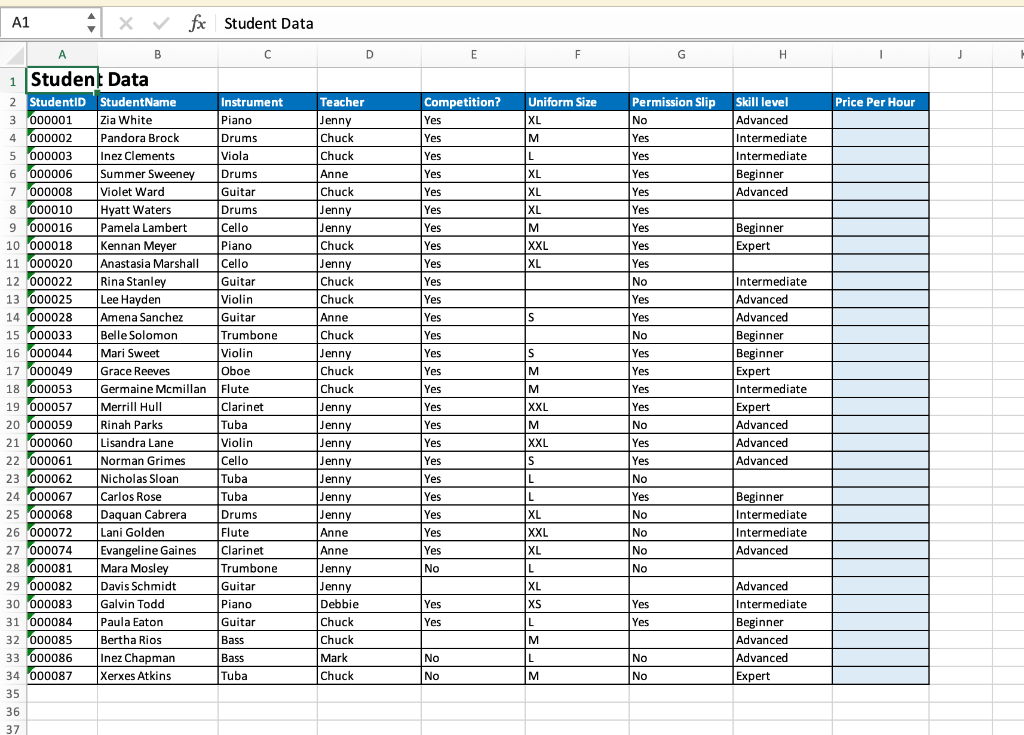
3	The StudentData worksheet contains data about each of Fiddlers student clients. The lesson price per hour varies based on the student's skill level. In cell I3, enter an INDEX function with a MATCH function to retrieve the lesson price for 1 hour, located in column 2 in the Lesson_Pricing named range, for each student on the basis of the students skill level, located in the Skill level field. To prevent an error from being displayed when the skill level is not known, use the IFERROR function to leave the cell blank. Copy the formula through cell I34.	7
4	Creating a named range for all of the student data will make it easier to retrieve data about each student in the table from other worksheets. On the StudentData worksheet, create a named range, Student_Data, for cells A3:I34.	3
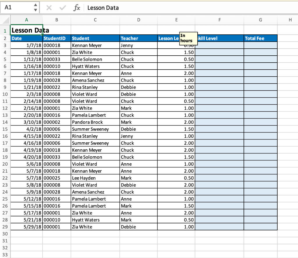
5	The LessonData worksheet contains the records for select students. However, their skill level is not included in the data set but is essential to calculate how much they owe for their lesson. In cell F3, enter a VLOOKUP function that will retrieve the skill level for the StudentID in cell B3 from the Student_Data named range. If the student does not have a skill level entered in the Student_Data named range, the VLOOKUP will return a value of 0. Incorporate an IF function in the formula so that if the value returned is a 0, display a blank value ("") instead, otherwise display the value returned by the VLOOKUP function. Copy the formula down through F29.	5
6	The cost of a lesson varies based on the length of the lesson and the skill level of the student. In cell G3, use INDEX and MATCH functions to retrieve the lesson fee for each student from the Lesson_Pricing named range. For the students with no skill level, a #N/A error will be returned. Incorporate an IFERROR function so that if an error is returned, the student is charged $50 for the lesson. Copy the formula down through G29.	10
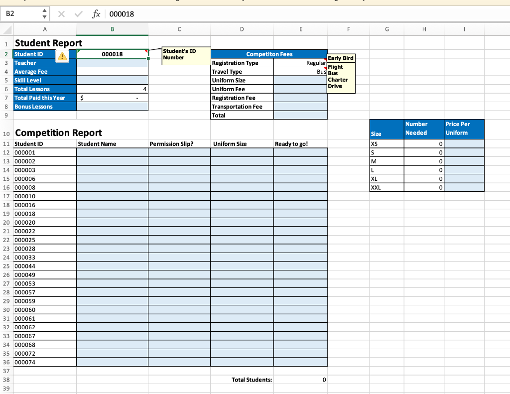
7	The Report worksheet is in need of some work for it to be fully functional. When a StudentID is entered into cell B2, the cells in B3:B8 should retrieve values about the student or calculate values pertaining to the student. In cell B3, enter a VLOOKUP function that will retrieve the teacher's name from the Student_Data named range for the StudentID entered in cell B2. Incorporate an IFERROR function to return a blank value ("") if there is no StudentID value in cell B2.	5
8	In cell B5, enter a VLOOKUP function that will retrieve the skill level from the Student_Data named range for the StudentID entered in cell B2. Incorporate an IFERROR function to return a blank value ("") if there is no StudentID value in cell B2.	5
9	Students at Fiddlers can start earning free lessons once they have taken more than 5. In cell B8, enter an IFS function to return 0 earned if the Total Lessons in cell B6 is less than 5, return 1 earned if the Total Lessons is less than 10, otherwise return 2 earned.	6
10	The CompetitionReport is in need of your help! The StudentIDs of those who are going on the road as part of the Fiddler's competition band have been provided in cells A12:A36. Starting in cell B12, enter a VLOOKUP function to retrieve the student's name from the Student_Data named range. Copy the formula down through B36.	5
11	In order for a student to go on the road with the band, they need to return a permission slip signed by their parent or guardian. In cell C12, enter a VLOOKUP to retrieve the value from the permission slip column in the Student_Data named range. Copy the formula down through C36.	5
12	The students going on the road need uniforms and the size they need is located in the Student_Data named range. In cell D12, enter a VLOOKUP function to retrieve the uniform size from the Student_Data named range. If there is no uniform size on record, a 0 will be returned. Incorporate an IF function so that if the value returned is 0, display a blank value (""), otherwise the VLOOKUP should return the uniform size. Copy the formula down through D36.	5
13	In order for a student to be ready to go on the road with the band, they need to have their permission slip returned and their uniform size on record. In cell E12, enter an IF function that will return Yes if there is a uniform size on record and a permission slip has been returned, otherwise return No. Copy the formula down through E34. Once completed, notice that in cell E38, the number of students ready to go has been calculated with a COUNTIF function.	5
14	Now that we have determined which students are going on the trip, you need to help calculate how much each of them must pay for their uniforms. The uniform shop has offered a sliding price scale, the more uniforms you buy of a particular size, the less expensive it is per person. In cell I11, enter an INDEX function to retrieve the per uniform price from the Uniform_Fees named range. You'll need to use a MATCH function that looks up the number of uniforms needed to determine the row number and another MATCH function that looks up the uniform size to determine the column number. Copy the formula down through I16.	10
15	The second half to the Student Report will retrieve the specific fees for which the student whose ID is in cell B2 is responsible. In cell E5, enter a VLOOKUP function that will retrieve the student's Uniform Size from the range A12:E36 on the StudentReport worksheet. Incorporate an IFERROR function so that if there is no Student ID in cell B2, a blank value ("") is returned instead of a #N/A error.	5
16	In cell E6, use a VLOOKUP function to retrieve the per uniform price from the range G11:I16 for the uniform size in cell E5.	5
17	In cell E7, use a HLOOKUP function to retrieve the Registration fee from the Entry_Fees named range based on the Registration Type in cell E3.	5
18	In cell E8, use an INDEX function to retrieve the Transportation Fee from the Trans_Fees named range based on the total number of students ready to go in cell E38 and the transportation mode in cell E4.	7
19	In cell E9, use a SUM function to calculate the total costs for which the student is responsible.	2
20	Save and close Excel_Ch05_Assessment_MusicLessons.xlsx. Exit Excel. Submit the file as directed.	0

\begin{tabular}{ll|llll} A1 & v & & fx & Student Data \end{tabular} \begin{tabular}{|l|r|l|} \hline Size & Number Needed & Price Per Unlform \\ \hline XS & 0 & \\ \hline S & 0 & \\ \hlineM & 0 & \\ \hline L & 0 & \\ \hline XL & 0 & \\ \hline XXL & 0 & \\ \hline \end{tabular} \begin{tabular}{ll|llll} A1 & v & & fx & Student Data \end{tabular} \begin{tabular}{|l|r|l|} \hline Size & Number Needed & Price Per Unlform \\ \hline XS & 0 & \\ \hline S & 0 & \\ \hlineM & 0 & \\ \hline L & 0 & \\ \hline XL & 0 & \\ \hline XXL & 0 & \\ \hline \end{tabular}