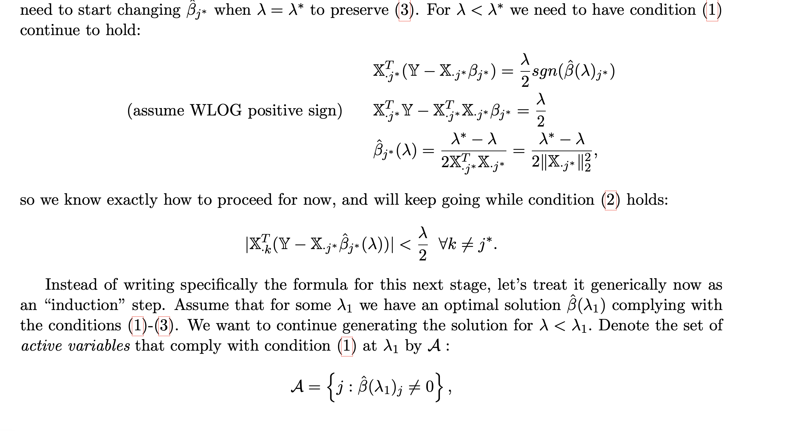
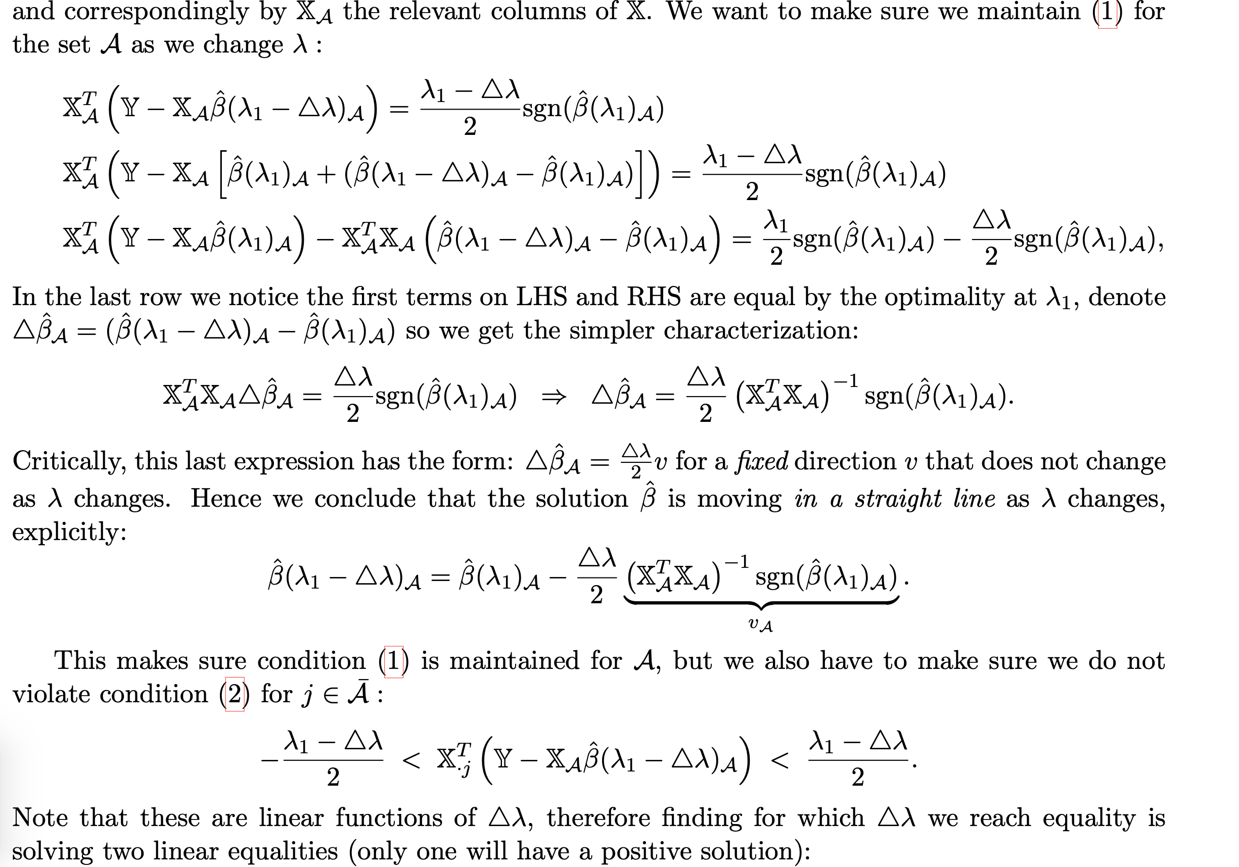
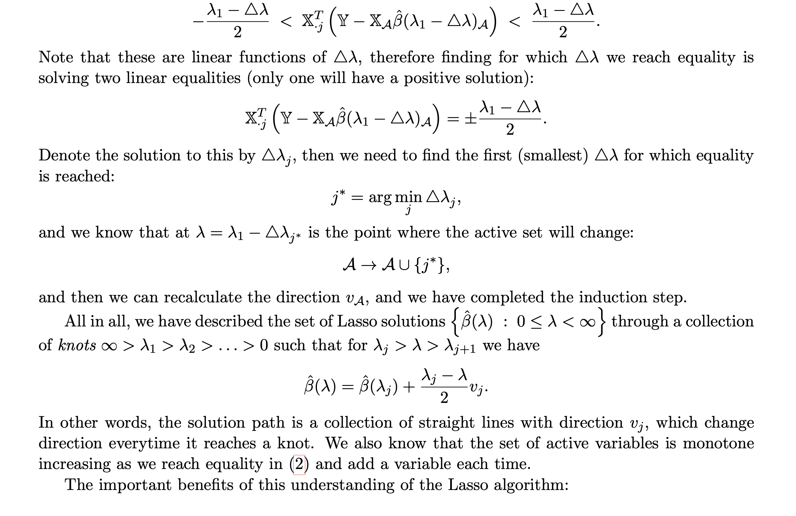
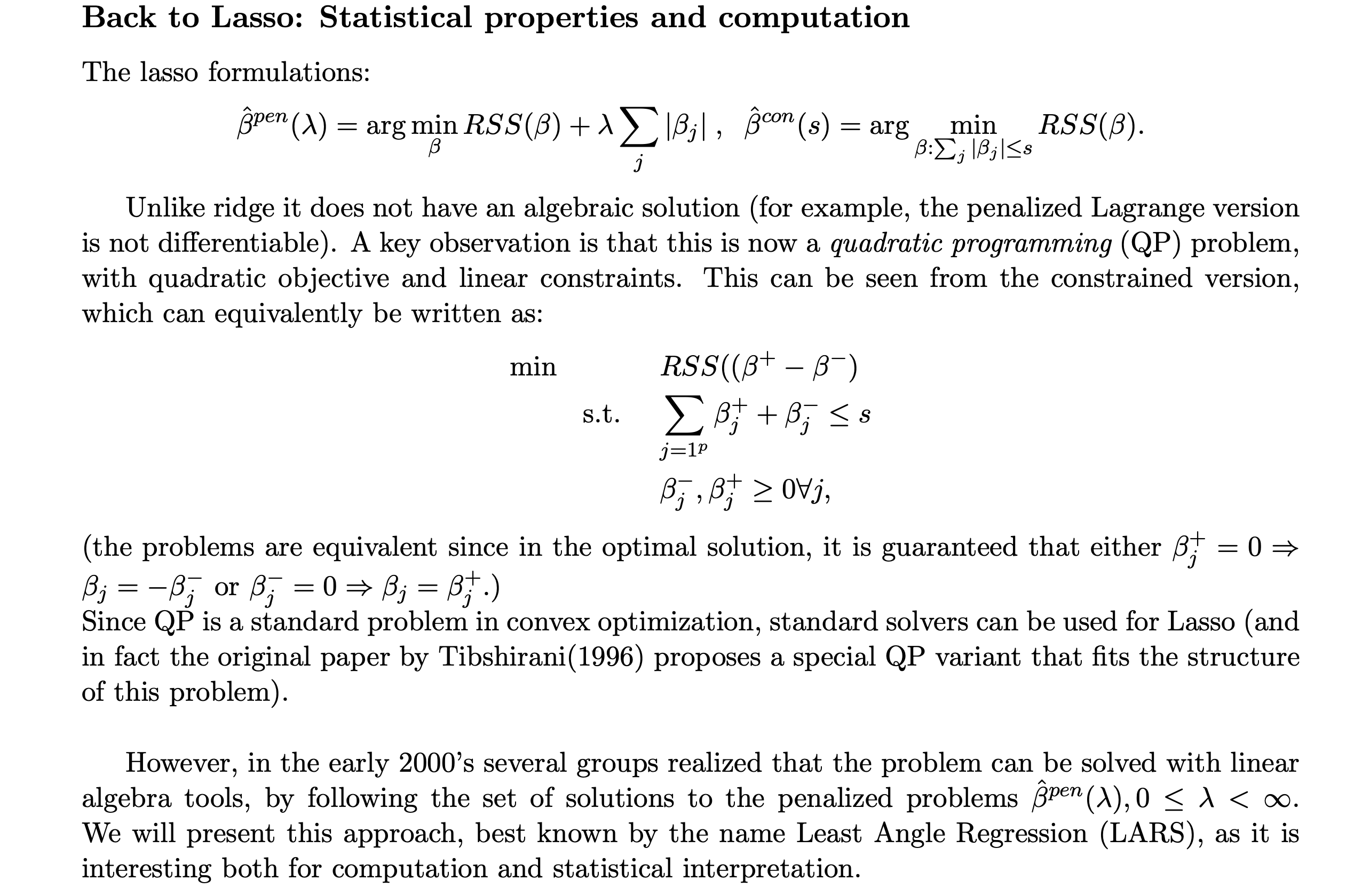
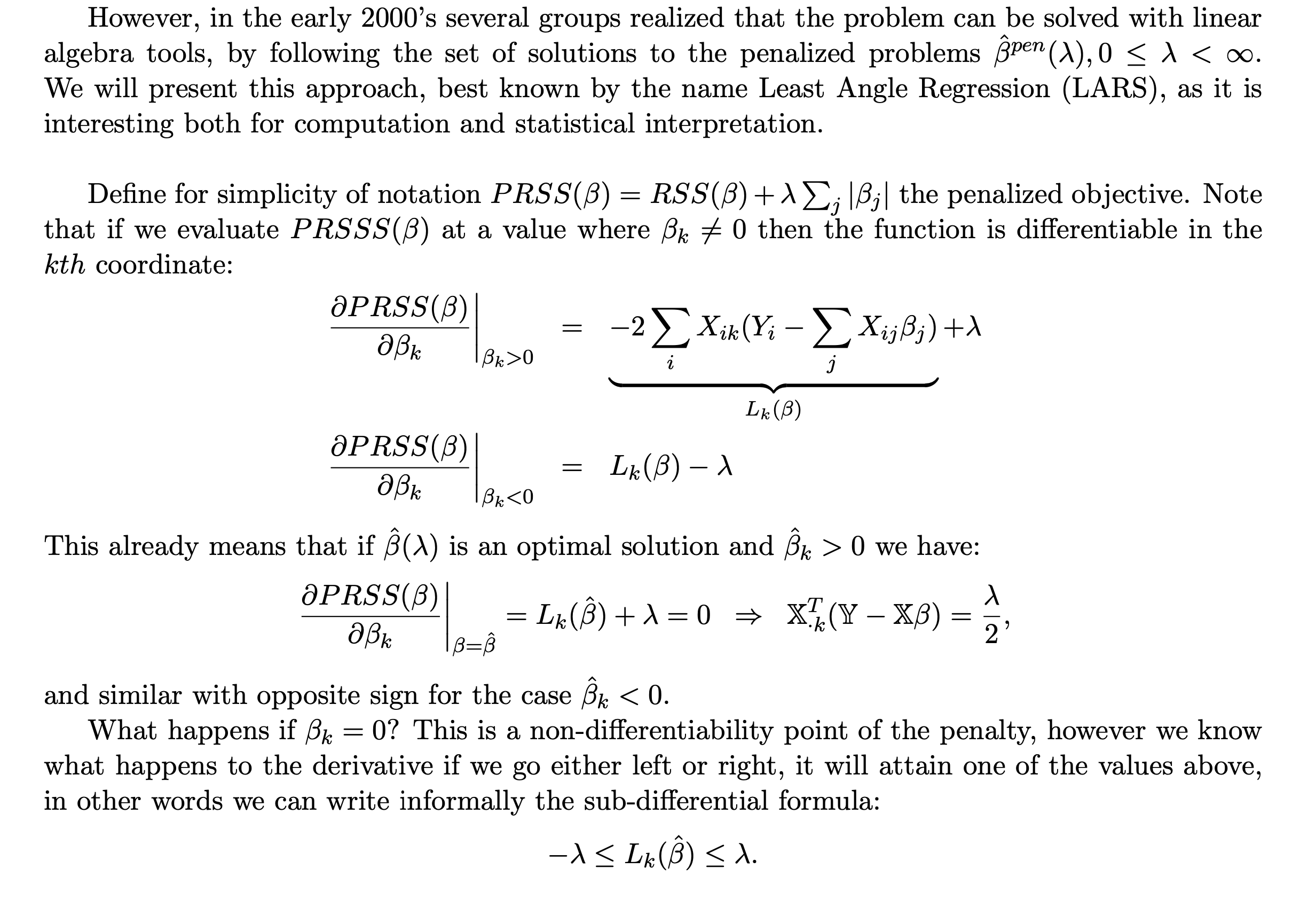
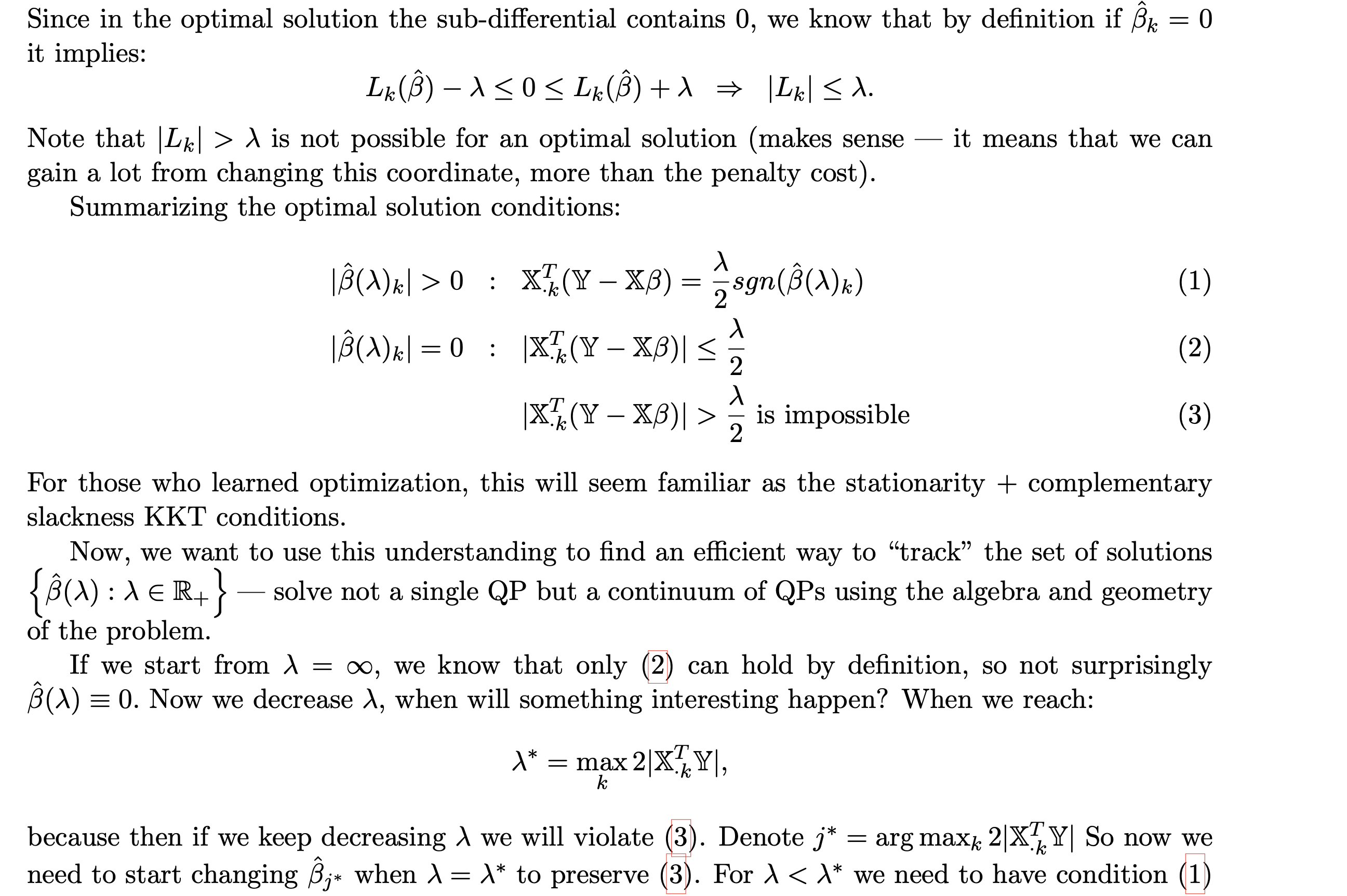
2. Which properties of Lasso path generalize to other loss functions? Recall we showed the optimality conditions for a Lasso solution: BN 0 > XE(Y XAN) = Ssen(BN)) 1) k=0 IXF(Y - XBO)| Ay > A2 > ... > {\\K > 0 such that the set A of active variables with non-zero coefficients is fixed for all solutions B(A) with Ax > A > Agy1. iii B(A) is a piecewise linear function, in other words, for A in this range we have: -~ BAA) = BO) + v\\ N), for a vector vy we explicitly derived in class. Assume now that we want to build a different type of model with a different convex and infinitely differentiable loss function, say a logistic regression model for a binary classification task, and add lasso penalty to that: B(A) = arg rrgnzlog {1+ exp{ysz] B}} + A|B|x- i=1 We would like to investigate which of the properties above still holds for the solution of this problem. (a) Using simple arguments about derivatives and sub-derivatives as we used in class for the quadratic loss case, argue that that three conditions like m-@ can be written for this case too, with the appropriate derivative replacing the empirical correlation. Derive these expressions explicitly for the logistic case. (b) Explain clearly why this implies that properties (i), (ii) still hold (for (ii), you may find the continuity of the derivative useful). (c) Does the piecewise linearity still hold? A clear intuitive explanation is sufficient here. Hint: Consider how we obtained the linearity for squared loss in AX in class by decomposing the correlation vector XT(Y XB3) = XTY XTX3. Back to Lasso: Statistical properties and computation The lasso formulations: BPen(N) :argmgnRSS +,\\Z|j B\""(s) =arg _min RSS(B). ,BZ]' 1Bj1 >; IBj| the penalized objective. Note that if we evaluate PRSSS(B) at a value where BK * 0 then the function is differentiable in the kth coordinate: OPRSS(B) = aBK -2 Xik( Yi - EXijBi) +d [ BK >0 i LK (B) OPRSS(B) = Lk(B) - > aBK IBK 0 we have: OPRSS(B) aBK = LK ( B) + 1 = 0 = X.H(Y - XB) =? IB=B and similar with opposite sign for the case BK A is not possible for an optimal solution (makes sense it means that we can gain a lot from changing this coordinate, more than the penalty cost). Summarizing the optimal solution conditions: BON >0+ XE(Y ~XB) = S sgn(BO) (1) B =0+ KLY -X8) % is impossible (3) For those who learned optimization, this will seem familiar as the stationarity + complementary slackness KKT conditions. Now, we want to use this understanding to find an efficient way to \"track\" the set of solutions { B N:Xxe R+} solve not a single QP but a continuum of QPs using the algebra and geometry of the problem. If we start from A = oo, we know that only (2) can hold by definition, so not surprisingly ,3 (A) = 0. Now we decrease A\\, when will something interesting happen? When we reach: X= m]?,X2|X,:',;Y|, because then if we keep decreasing A we will violate @) Denote j* = arg maxy 2|X.:',;Y| So now we need to start changing Bj* when A = \\* to preserve ( ) For A * we need to have condition (1) continue to hold: X.;* (Y - X.j*Bj* ) = sgn(B(X);*) (assume WLOG positive sign) Bj * ( 1 ) = _ * * - * 1* - 1 2X74X.jx 2 1X.,* 113 so we know exactly how to proceed for now, and will keep going while condition (2) holds: X H( Y - X. jx Bj *(X))I1. Denote the set of active variables that comply with condition (1) at 1 by A : A = { j : B(1 );to),and correspondingly by XA the relevant columns of X. We want to make sure we maintain (1) for the set A as we change 1 : XX (Y - XAB()1 - AN)A) = 1 - AX 2 - sgn (B(1)A) XAY - XA B(1)A+ (B(X1 - AN)A-B(21)A)): 2 sgn(B(1)A) XA (Y - XAB(1)A) - XAXA ( B(M - ANA - B(1)A) = 2 son( B(1)A) -2sen( 8(1 )A ) , In the last row we notice the first terms on LHS and RHS are equal by the optimality at 1, denote ABA = (8()1 - AX)A - B()1)A) so we get the simpler characterization: XXAABA = 4 2 son ( B ( 1 ) A ) = ABA = 2 (X4XA) son( B(1)A). Critically, this last expression has the form: ABA = 2v for a fixed direction v that does not change as A changes. Hence we conclude that the solution / is moving in a straight line as A changes, explicitly: B( Al - AN)A = B(1)A - (XXXA) son(B(1)A) . U A This makes sure condition (1) is maintained for A, but we also have to make sure we do not violate condition (2) for j E A : 2 A1 > A2 > ... > 0 such that for A; > XA > A; 1 we have = A Ai A BOY = B0y) + L In other words, the solution path is a collection of straight lines with direction v;, which change direction everytime it reaches a knot. We also know that the set of active variables is monotone increasing as we reach equality in (2) and add a variable each time. The important benefits of this understanding of the Lasso algorithm: Uj