21

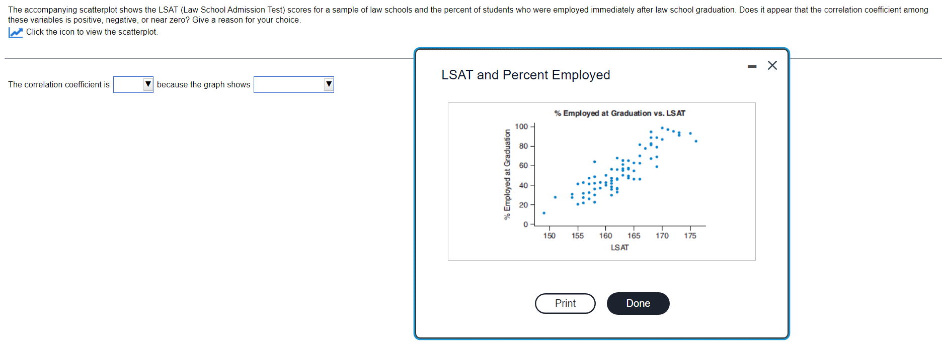
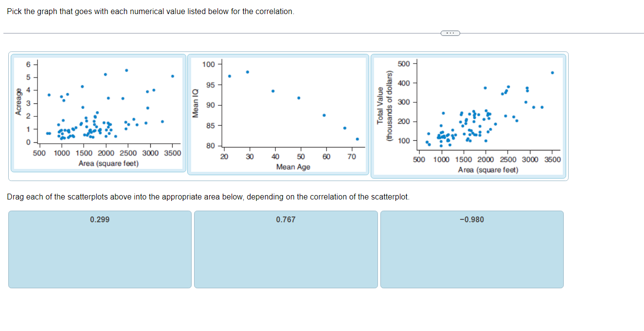
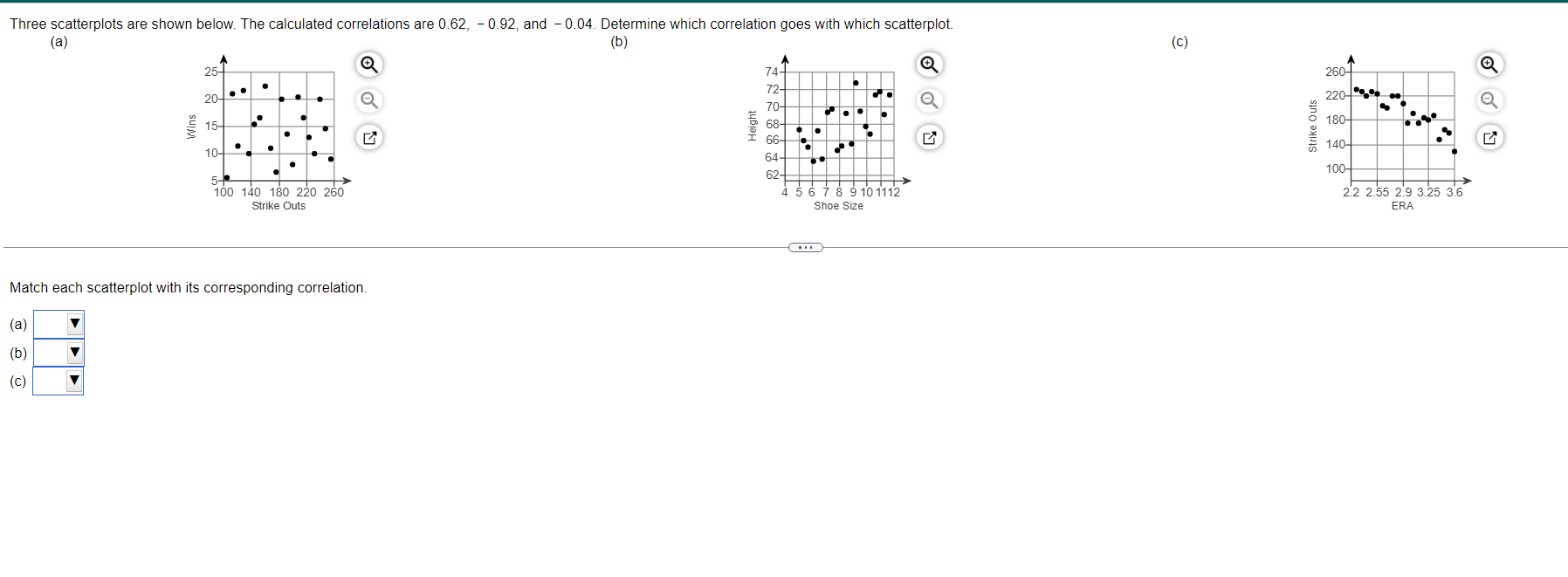
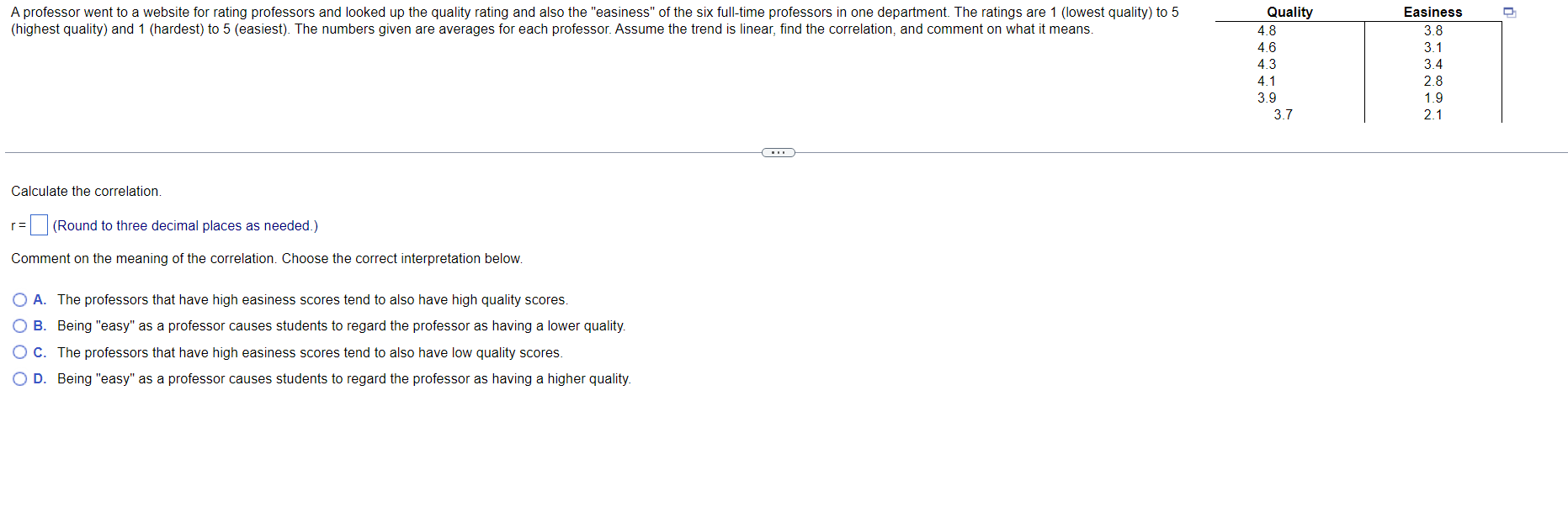
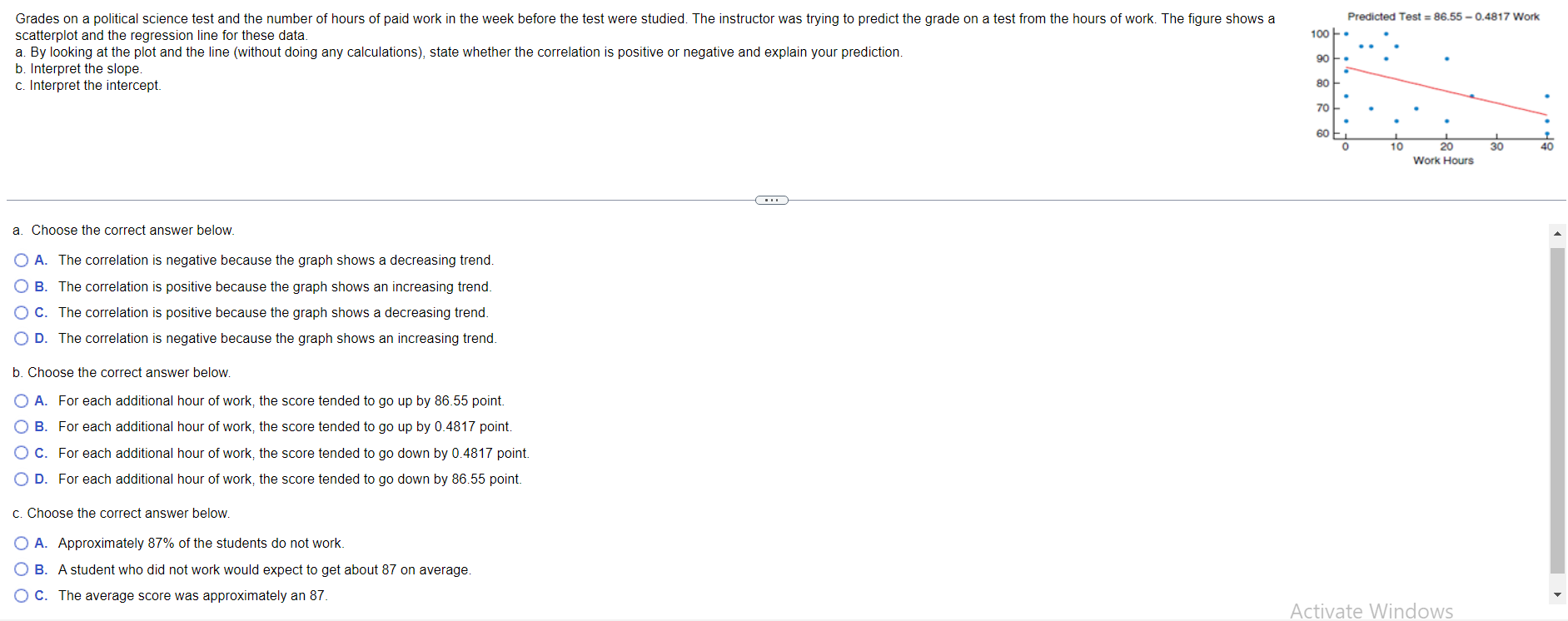
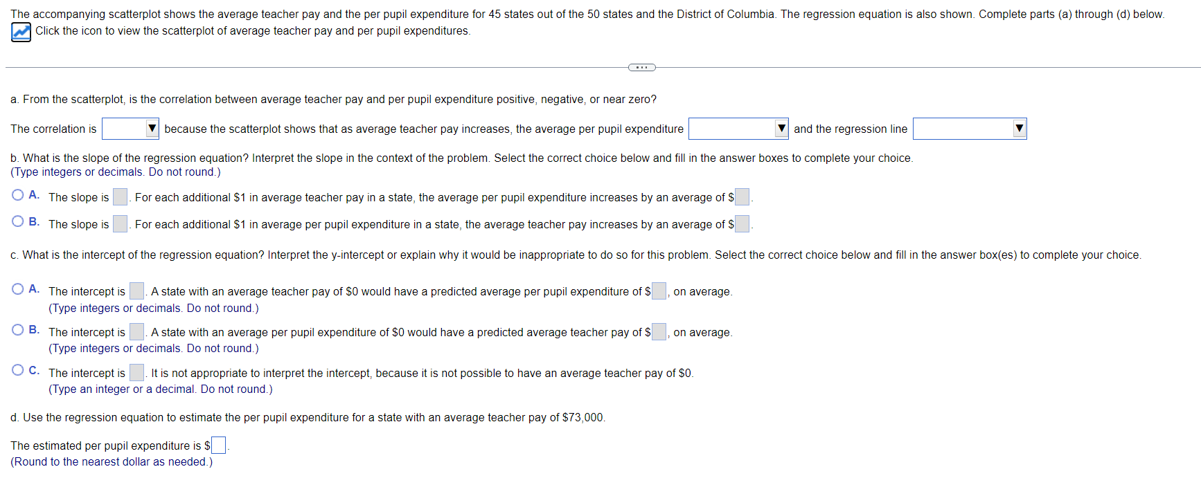
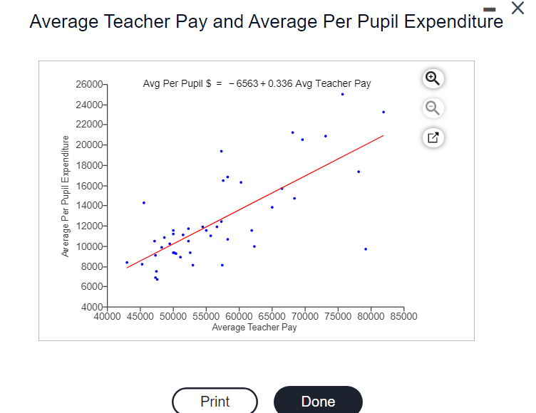
The accompanying scatterplot shows the LSAT (Law School Admission Test) scores for a sample of law schools and the percent of students who were employed immediately after law school graduation. Does it appear that the correlation coefficient among these variables is positive, negative, or near zero? Give a reason for your choice. Click the icon to view the scatterplot. - X LSAT and Percent Employed The correlation coefficient is because the graph shows % Employed at Graduation vs. LSAT 100 - .. . 5 80 - 60 - % Employed at Graduation 40 - 20 150 155 160 165 170 175 LSAT Print DonePick the graph that goes with each numerical value listed below for the correlation. am 1om1soom 2500 soon moo Antwan-Ital) Drag each of the scatterplots above into the appropriate area below, depending on the correlation of the scatterplot, Three scatterplots are shown below. The calculated correlations are 0.62, - 0.92, and - 0.04. Determine which correlation goes with which scatterplot. (a) (b) (c) 25- 74 260- 72- 20- 220- 70- 180 leight 68- Strike Outs 66- 140- 10 64- 100- 5- 62- 100 140 180 220 260 4 5 6 7 8 9 10 1112 2.2 2.55 2.9 3.25 3.6 Strike Outs Shoe Size ERA Match each scatterplot with its corresponding correlation. (a)A professor went to a website for rating professors and looked up the quality rating and also the "easiness" of the six full-time professors in one department. The ratings are 1 (lowest quality) to 5 Quality Easiness (highest quality) and 1 (hardest) to 5 (easiest). The numbers given are averages for each professor. Assume the trend is linear, find the correlation, and comment on what it means. 4.8 3.8 1.6 3.1 4.3 3.4 4.1 2.8 39 1.9 3.7 2.1 Calculate the correlation. r=(Round to three decimal places as needed.) Comment on the meaning of the correlation. Choose the correct interpretation below. O A. The professors that have high easiness scores tend to also have high quality scores. O B. Being "easy" as a professor causes students to regard the professor as having a lower quality. O C. The professors that have high easiness scores tend to also have low quality scores. O D. Being "easy" as a professor causes students to regard the professor as having a higher quality.Grades on a political science test and the number of hours of paid work In the week before the test were studied. The instructor was trying to predict the grade on a test from the hours of work. The gure shows a m TO! = 3955 - "15'7"\" scatterplot and the regression line for these data 100 a Ely looking at the plot and the line (Without doing any calculations), state whether the correlation is positive or negative and explain your prediction. b interpret the slope c. Interpret the intercept 8388 a Choose the correct answer below A O A. The correlation is negative because the graph shows a decreasing trend. 0 E. The correlation is positive because the graph shows an increasing trend. O C. The correlation is positive because the graph shows a decreasing trend 0 D. The correlation is negative because the graph shows an increasing trend. b Choose the correm answer below O A. For each additional hour of work, the score tended to go up by 86.55 point. O E. For each additional hour of work, the score tended to go up by 0 4817 point O c. For each additional hour of work, the score tended to go down by 04817 point O D. For each additional hour of work, the score tended to go down by 86.55 point C Choose the correct answer DSIOW. O A. Approximately 87% ot the students do not work O E. A student who did not work would expect to get about 87 on average O C. The average score was approximately an 87. . . v Activate Windows The accompanying scatterplot shows the average teacher pay and the per pupil expenditure for 45 states out of the 50 states and the District otColumbia. The regressmn equation is also shown. Complete parts (a) through (d) below. a Click the icon to View the scatterplot of average teacher pay and per pupil expenditures. a. From the scatterplot, is the correlation between average teacher pay and per pupil expenditure positive, negative, or near zero? The correlation is V because the scatterplot shows that as average teacher pay increases, the average per pupil expenditure V and the regression line V b. What is the slope ofthe regression equation? Interpret the slope in the context of the problem Select the correct choice below and ll in the answer boxes to complete your choice. (Type integers or decimals. Do not round ) O A- The slope is . For each additional $1 in average teacher pay in a state, the average per pupil expenditure increases by an average of $ O E- The slope is . For each additional $1 in average per pupil expenditure in a state, the average teacher pay increases by an average of $ c What is the intercept of the regression equation?l interpret the yiintercept or explain why it would be inappropriate to do so for this problem. Select the correct ch0ice below and ll in the answer box(es) to complete your choice. O A- The intercept is . A state with an average teacher pay of $0 would have a predicted average per pupil expenditure of$ , on average. (Type integers or deCImals. Do not round.) O E- The intercept is A state with an average per pupil expenditure of $0 would have a predicted average teacher pay of$ , on average (Type integers or deCImals Do not round.) O C- The intercept is It is not appropriate to interpret the intercept, because it is not possible to have an average teacher pay of $0. (Type an integer or a decimal. Do not round.) d. Use the regression equation to estimate the per pupil expenditure for a state with an average teacher pay of $73,000. The estimated per pupil expenditure is $ (Round to the nearest dollar as needed.) X Average Teacher Pay and Average Per Pupil Expenditure 26000- Avg Per Pupil $ = - 6563 + 0.336 Avg Teacher Pay 24000- 22000- 20000- 18000- 16000- Average Per Pupil Expenditure 14000- 12000- 10000- 8000- 6000- 4000- 40000 45000 50000 55000 60000 65000 70000 75000 80000 85000 Average Teacher Pay Print Done