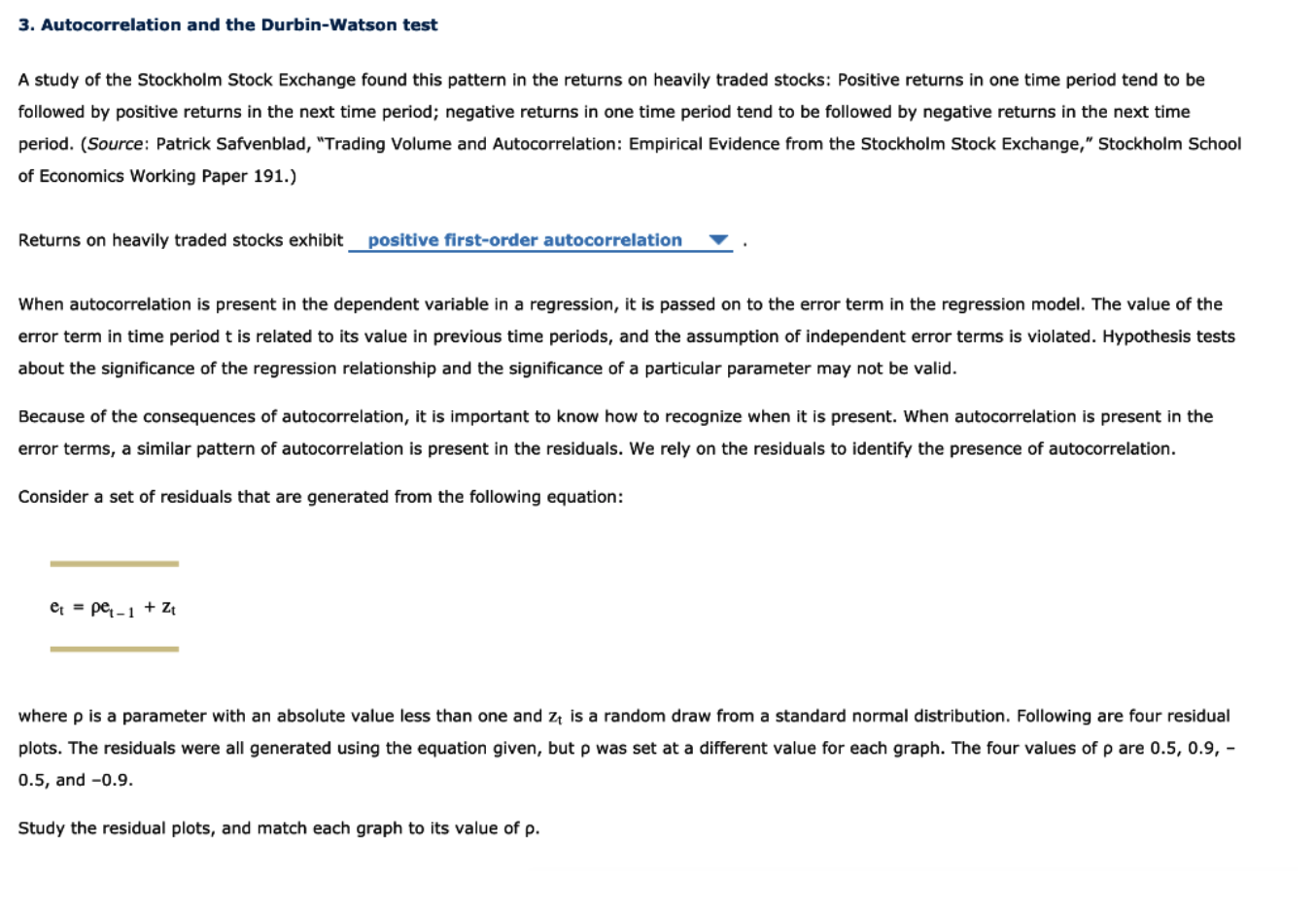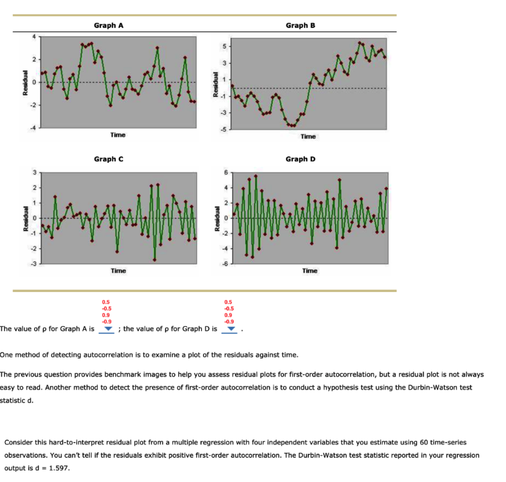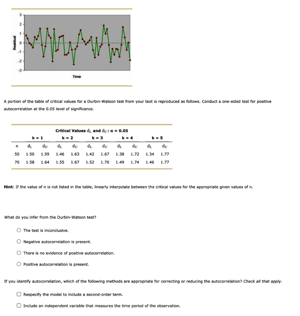
3. Autocorrelation and the Durbin-Watson test A study of the Stockholm Stock Exchange found this pattern in the returns on heavily traded stocks: Positive returns in one time period tend to be followed by positive returns in the next time period; negative returns in one time period tend to be followed by negative returns in the next time period. (Source: Patrick Safvenblad, "Trading Volume and Autocorrelation: Empirical Evidence from the Stockholm Stock Exchange," Stockholm School of Economics Working Paper 191.) Returns on heavily traded stocks exhibit positive first-order autocorrelation When autocorrelation is present in the dependent variable in a regression, it is passed on to the error term in the regression model. The value of the error term in time period t is related to its value in previous time periods, and the assumption of independent error terms is violated. Hypothesis tests about the significance of the regression relationship and the significance of a particular parameter may not be valid. Because of the consequences of autocorrelation, it is important to know how to recognize when it is present. When autocorrelation is present in the error terms, a similar pattern of autocorrelation is present in the residuals. We rely on the residuals to identify the presence of autocorrelation. Consider a set of residuals that are generated from the following equation: e = pe-1 + Zt where p is a parameter with an absolute value less than one and zt is a random draw from a standard normal distribution. Following are four residual plots. The residuals were all generated using the equation given, but p was set at a different value for each graph. The four values of p are 0.5, 0.9,- 0.5, and -0.9. Study the residual plots, and match each graph to its value of p. Graph A Graph B 2 3 Arthur 0 -2 Time Time Graphc Graph D 2 -1 -3 Time Time 0.5 -0.5 0.9 -0.9 -0.5 0.9 -0.9 The value of p for Graph A is ; the value of p for Graph D is One method of detecting autocorrelation is to examine a plot of the residuals against time. The previous question provides benchmark images to help you assess residual plots for first-order autocorrelation, but a residual plot is not always easy to read. Another method to detect the presence of first-order autocorrelation is to conduct a hypothesis test using the Durbin-Watson test statistic d. Consider this hard-to-interpret residual plot from a multiple regression with four independent variables that you estimate using 60 time-series observations. You can't tell if the residuals exhibit positive first-order autocorrelation. The Durbin-Watson test statistic reported in your regression output is d = 1.597. 3 2 1 0 Way MA -2 Time A portion of the table of critical values for a Durbin-Watson test from your text is reproduced as follows. Conduct a one-sided test for positive autocorrelation at the 0.05 level of significance. Critical Values dl and du: a = 0.05 k = 2 k = 3 k = 4 k = 1 k = 5 n dL du dL du dL du dL du dL du 1.77 50 1.50 1.59 1.46 1.63 1.42 1.67 1.38 1.72 1.34 70 1.58 1.64 1.55 1.67 1.52 1.70 1.49 1.74 1.46 1.77 Hint: If the value of n is not listed in the table, linearly interpolate between the critical values for the appropriate given values of n. What do you infer from the Durbin-Watson test? O The test is inconclusive. O Negative autocorrelation is present. There is no evidence of positive autocorrelation. O Positive autocorrelation is present. If you identify autocorrelation, which of the following methods are appropriate for correcting or reducing the autocorrelation? Check all that apply. Respecify the model to include a second-order term. Include an independent variable that measures the time period of the observation. 3. Autocorrelation and the Durbin-Watson test A study of the Stockholm Stock Exchange found this pattern in the returns on heavily traded stocks: Positive returns in one time period tend to be followed by positive returns in the next time period; negative returns in one time period tend to be followed by negative returns in the next time period. (Source: Patrick Safvenblad, "Trading Volume and Autocorrelation: Empirical Evidence from the Stockholm Stock Exchange," Stockholm School of Economics Working Paper 191.) Returns on heavily traded stocks exhibit positive first-order autocorrelation When autocorrelation is present in the dependent variable in a regression, it is passed on to the error term in the regression model. The value of the error term in time period t is related to its value in previous time periods, and the assumption of independent error terms is violated. Hypothesis tests about the significance of the regression relationship and the significance of a particular parameter may not be valid. Because of the consequences of autocorrelation, it is important to know how to recognize when it is present. When autocorrelation is present in the error terms, a similar pattern of autocorrelation is present in the residuals. We rely on the residuals to identify the presence of autocorrelation. Consider a set of residuals that are generated from the following equation: e = pe-1 + Zt where p is a parameter with an absolute value less than one and zt is a random draw from a standard normal distribution. Following are four residual plots. The residuals were all generated using the equation given, but p was set at a different value for each graph. The four values of p are 0.5, 0.9,- 0.5, and -0.9. Study the residual plots, and match each graph to its value of p. Graph A Graph B 2 3 Arthur 0 -2 Time Time Graphc Graph D 2 -1 -3 Time Time 0.5 -0.5 0.9 -0.9 -0.5 0.9 -0.9 The value of p for Graph A is ; the value of p for Graph D is One method of detecting autocorrelation is to examine a plot of the residuals against time. The previous question provides benchmark images to help you assess residual plots for first-order autocorrelation, but a residual plot is not always easy to read. Another method to detect the presence of first-order autocorrelation is to conduct a hypothesis test using the Durbin-Watson test statistic d. Consider this hard-to-interpret residual plot from a multiple regression with four independent variables that you estimate using 60 time-series observations. You can't tell if the residuals exhibit positive first-order autocorrelation. The Durbin-Watson test statistic reported in your regression output is d = 1.597. 3 2 1 0 Way MA -2 Time A portion of the table of critical values for a Durbin-Watson test from your text is reproduced as follows. Conduct a one-sided test for positive autocorrelation at the 0.05 level of significance. Critical Values dl and du: a = 0.05 k = 2 k = 3 k = 4 k = 1 k = 5 n dL du dL du dL du dL du dL du 1.77 50 1.50 1.59 1.46 1.63 1.42 1.67 1.38 1.72 1.34 70 1.58 1.64 1.55 1.67 1.52 1.70 1.49 1.74 1.46 1.77 Hint: If the value of n is not listed in the table, linearly interpolate between the critical values for the appropriate given values of n. What do you infer from the Durbin-Watson test? O The test is inconclusive. O Negative autocorrelation is present. There is no evidence of positive autocorrelation. O Positive autocorrelation is present. If you identify autocorrelation, which of the following methods are appropriate for correcting or reducing the autocorrelation? Check all that apply. Respecify the model to include a second-order term. Include an independent variable that measures the time period of the observation