

Question
3 files for data Augusta Location Category 1st Quarter 2nd Quarter 3rd Quarter 4th Quarter Total Dine-In $ 40,000 $ 34,000 $ 29,000 $ 22,000
3 files for data
| Augusta Location | |||||
| Category | 1st Quarter | 2nd Quarter | 3rd Quarter | 4th Quarter | Total |
| Dine-In | $ 40,000 | $ 34,000 | $ 29,000 | $ 22,000 | $ 125,000 |
| Pick-up | $ 62,000 | $ 63,000 | $ 62,000 | $ 63,000 | $ 250,000 |
| Delivery | $ 22,000 | $ 26,000 | $ 35,000 | $ 42,000 | $ 125,000 |
| Total | $ 124,000 | $ 123,000 | $ 126,000 | $ 127,000 | $ 500,000 |
| Lewiston Location | |||||
| Category | 1st Quarter | 2nd Quarter | 3rd Quarter | 4th Quarter | Total |
| Dine-In | $ 12,000 | $ 10,000 | $ 8,000 | $ 6,000 | $ 36,000 |
| Pick-up | $ 27,000 | $ 26,000 | $ 26,000 | $ 26,000 | $ 105,000 |
| Delivery | $ 25,000 | $ 34,000 | $ 46,000 | $ 60,000 | $ 165,000 |
| Total | $ 64,000 | $ 70,000 | $ 80,000 | $ 92,000 | $ 306,000 |
| Portland Location | |||||
| Category | 1st Quarter | 2nd Quarter | 3rd Quarter | 4th Quarter | Total |
| Dine-In | $ 45,000 | $ 41,000 | $ 38,000 | $ 33,000 | $ 157,000 |
| Pick-up | $ 19,000 | $ 21,000 | $ 20,000 | $ 20,000 | $ 80,000 |
| Delivery | $ 25,000 | $ 35,000 | $ 45,000 | $ 55,000 | $ 160,000 |
| Total | $ 89,000 | $ 97,000 | $ 103,000 | $ 108,000 | $ 397 |
Main file by teacher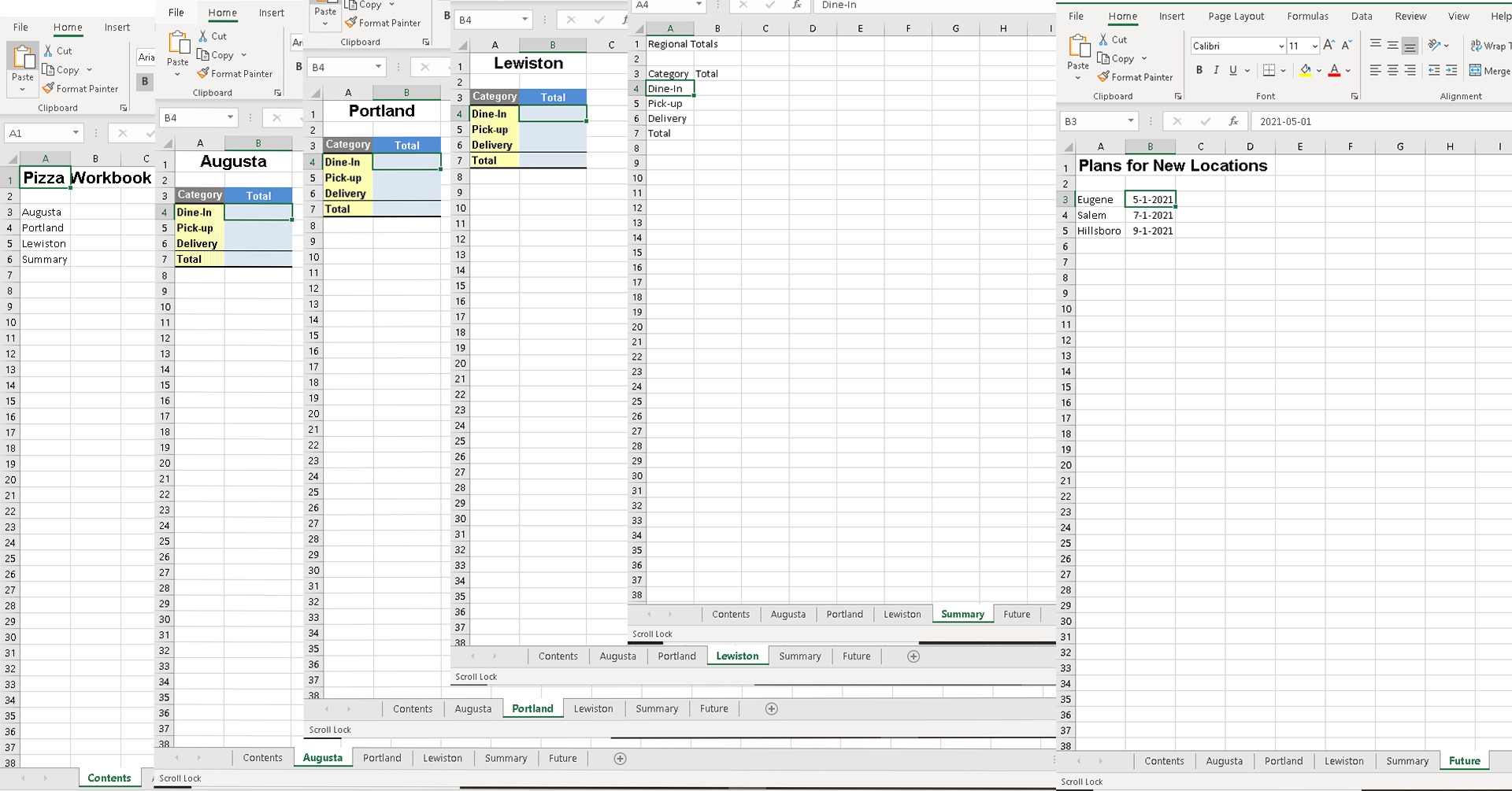
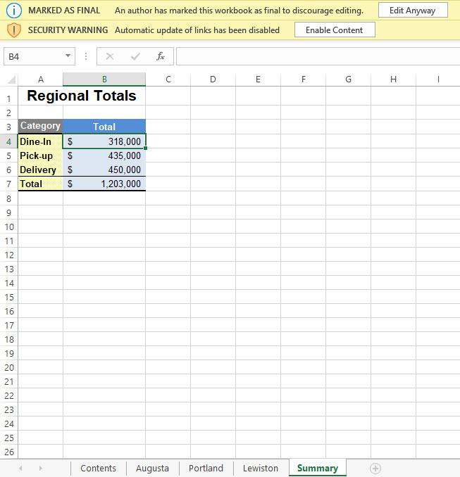
Final result image by teacher
I can send the excel files. please give me a email thank you
-the first image is the questions to solve
-then the 3 below it are the data to use
-then the file teacher provided to do the work on
-and last the final result image teacher provided
Please help Thank you
and the pictures are clear if you open them in new tab sir/madam. i gave the whole answer as it was in the documents provided by the teacher. i missed the dead line so never mind now. not really helpfull
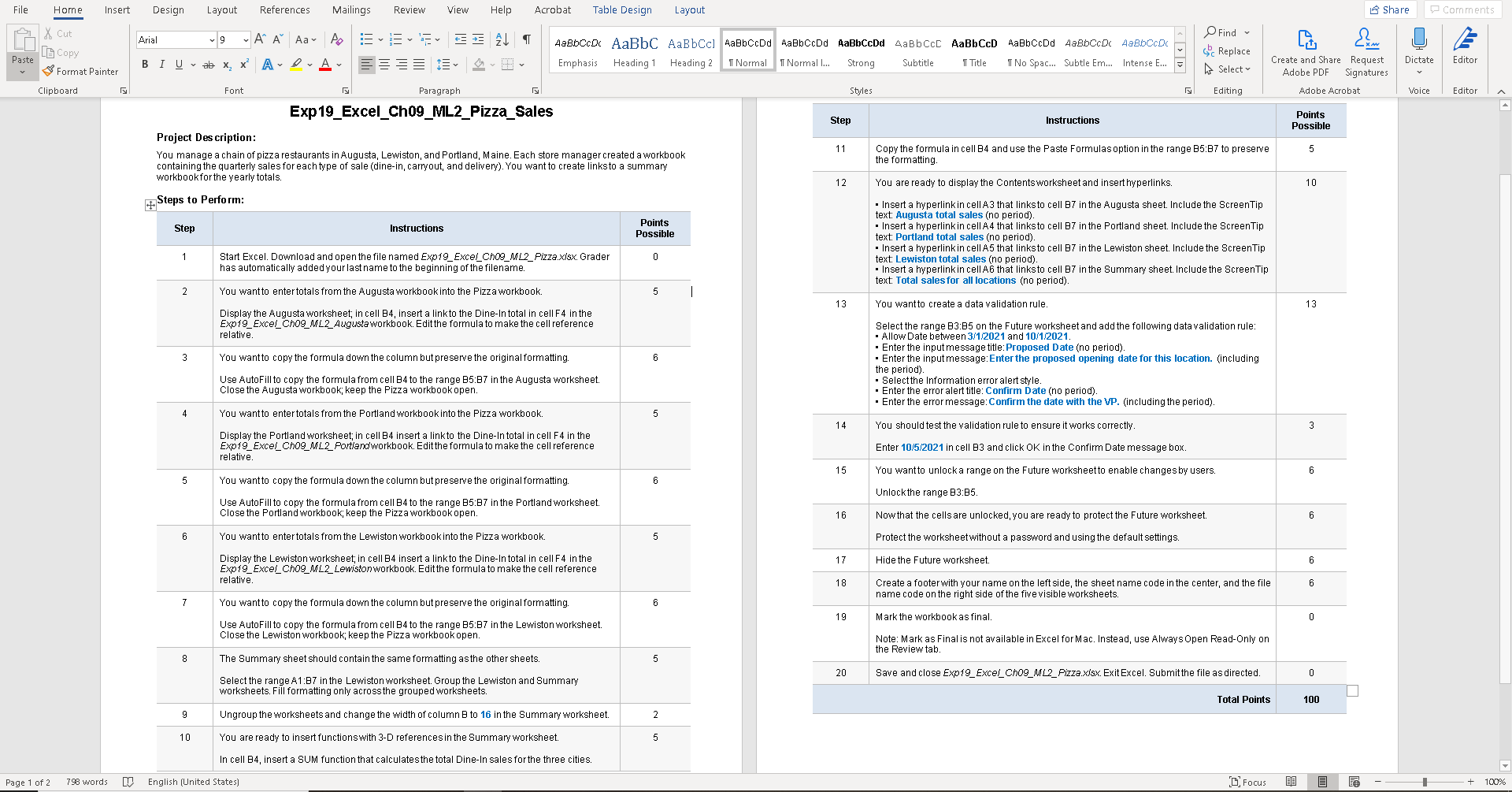
File Home Insert Design Layout References Mailings Review View Help Acrobat Table Design Layout Share Comments Arial 9 ~ A Aa AO JT X Cut Copy * Format Painter Find Replace Select AaBDCD AaBbC AaBbCcl AaBbccd AaBbccd AaBhCcDd AaBbccc AaBbCcD AaBbccd AaBbccDc AaBbccdc Emphasis Heading 1 Heading 2 I Normal T Normal ... Strong Subtitle I Title I No Spac... Subtle Em... Intense E... Paste BIUb X, X A Dictate Editor Create and Share Request Adobe PDF Signatures Adobe Acrobat Clipboard Styles Editing Voice Editor Step Instructions Points Possible Font Paragraph Exp19_Excel_Ch09_ML2_Pizza_Sales Project Description: You manage a chain of pizza restaurants in Augusta, Lewiston, and Portland, Maine. Each store manager created a workbook containing the quarterly sales for each type of sale (dine-in, carryout, and delivery). You want to create linksto a summary workbookfor the yearly totals. 11 Copy the formula in cell B4 and use the Paste Formulas option in the range B5:87 to preserve the formatting 5 12 10 Steps to Perform: Step Instructions Points Possible You are ready to display the Contentsworksheet and insert hyperlinks. Insert a hyperlinkin cell A3 that linksto cell B7 in the Augusta sheet. Include the ScreenTip text: Augusta total sales (no period). Insert a hyperlink in cell A4 that linksto cell B7 in the Portland sheet. Include the Screen Tip text: Portland total sales (no period). Insert a hyperlinkin cell A5 that linksto cell B7 in the Lewiston sheet. Include the ScreenTip text: Lewiston total sales (no period). Insert a hyperlink in cell A6 that linksto cell B7 in the Summary sheet. Include the ScreenTip text: Total sales for all locations (no period). 1 0 Start Excel. Download and open the file named Exp19_Excel_Ch09_ML2_Pizza.xlsx. Grader has automatically added your last name to the beginning of the filename. You want to enter totals from the Augusta workbook into the Pizza workbook. 2 5 | 13 You want to create a data validation rule. 13 Display the Augusta worksheet; in cell B4, insert a link to the Dine-In total in cell F4 in the Exp19_ExcelChog_ML2_Augusta workbook. Edit the formula to make the cell reference relative. 3 You want to copy the formula down the column but preserve the originalformatting. 6 Select the range B3:85 on the Future worksheet and add the following data validation rule: . Allow Date between 3/1/2021 and 10/1/2021. Enter the input message title: Proposed Date (no period). Enter the input message: Enter the proposed opening date for this location. (including the period) Select the Information error alert style. - Enter the error alert title: Confirm Date (no period). Enter the error message: Confirm the date with the VP. (including the period). Use AutoFill to copy the formula from cell B4 to the range B5:87 in the Augusta worksheet. Close the Augusta workbook; keep the Pizza workbookopen. 4 You wantto enter totals from the Portland workbook into the Pizza workbook. 5 14 You should test the validation rule to ensure it works correctly. 3 Display the Portland worksheet; in cell B4 insert a link to the Dine-In total in cell F4 in the Exp19_Excel_Ch09_ML2_ Portlandworkbook. Edit the formula to make the cell reference relative. Enter 10/5/2021 in cell B3 and click OK in the Confirm Date message box. 15 You want to unlocka range on the Future worksheetto enable changes by users. 6 5 6 You want to copy the formula down the column but preserve the original formatting. Use AutoFill to copy the formula from cell B4 to the range 85:87 in the Portland worksheet. Close the Portland workbook, keep the Pizza workbook open. Unlock the range B3:05. 16 Now that the cells are unlocked, you are ready to protect the Future worksheet. 6 6 You wantto enter totals from the Lewiston workbook into the Pizza workbook. 5 Protect the worksheet without a password and using the default settings. 17 Hide the Future worksheet 6 Display the Lewiston worksheet; in cell B4 insert a link to the Dine-In total in cell F4 in the Exp19_Excel_Chog_ML2_Lewistonworkbook. Edit the formula to make the cell reference relative. 18 6 Create a footer with your name on the left side, the sheet name code in the center, and the file name code on the right side of the five visible worksheets. 7 6 You want to copy the formula down the column but preserve the originalformatting. Use AutoFill to copy the formula from cell B4 to the range B5:37 in the Lewiston worksheet. Close the Lewiston workbook; keep the Pizza workbook open. 19 Mark the workbook as final. 0 Note: Mark as Finalis not available in Excel for Mac. Instead, use Always Open Read-Only on the Review tab. 8 5 The Summary sheet should contain the same formatting as the other sheets. Select the range A1:87 in the Lewiston worksheet. Group the Lewiston and Summary worksheets. Fill formatting only across the grouped worksheets. 20 Save and close Exp19_Excel_Ch09_ML2_Pizza.xlsx. Exit Excel. Submit the file as directed. 0 Total Points 100 9 Ungroup the worksheets and change the width of column B to 16 in the Summary worksheet. 2 10 You are ready to insert functions with 3-D references in the Summary worksheet. 5 In cell B4, insert a SUM function that calculates the total Dine-In sales for the three cities. Page 1 of 2 796 words m English (United States) C) Focus 100% A4 fix Dine-In File Home Insert Paste - Copy B File Home Insert Page Layout Formulas Data Review View Help File B4 Home Insert Format Painter D E F G H 1 An Clipboard C Calibri = ab Wrap Aria X Cut LG Copy Format Painter Paste X Cut [Copy vStep by Step Solution
There are 3 Steps involved in it
Step: 1

Get Instant Access to Expert-Tailored Solutions
See step-by-step solutions with expert insights and AI powered tools for academic success
Step: 2

Step: 3
Ace Your Homework with AI
Get the answers you need in no time with our AI-driven, step-by-step assistance
Get Started
Foreign Direct Investment Smart Approaches To Differentiation And Engagement
Authors: Daniel Nicholls
1st Edition
1409423573,1409471381