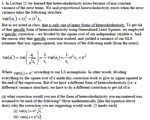
3. In Lecture 11 we learned that heteroskedasticity arises because of non-constant variance of the error terms. We said proportional heteroskedasticity exists when the error variance takes the following structure: var (e,)= =x But as we noted in class, that is only one of many forms of heteroskedasticity. To get rid of that specific form of heteroskedasticity using Generalized Least Squares, we employed a specific correction - we divided by the square root of our independent variable x. And the reason why that specific correction worked, and yielded a variance of our GLS estimates that was sigma-squared, was because of the following math (from the notes): var(e) = var 1 var(e) 10x = 0 x x Where var(e,)=0 according to our LS assumptions. In other words, dividing everything by the square root of x made this correction work to give us sigma squared at the end of the expression. But if we have a different form of heteroskedasticity (i.e. a difference variance structure), we have to do a different correction to get rid of it. (a) what correction would you use if the form of heteroskedasticity you encountered was assumed to be each of the following? Show mathematically (like the equation above does) why the correction you are suggesting would work. (5 marks each) (1) var(e,)=x, (ii) var(e,)=0x