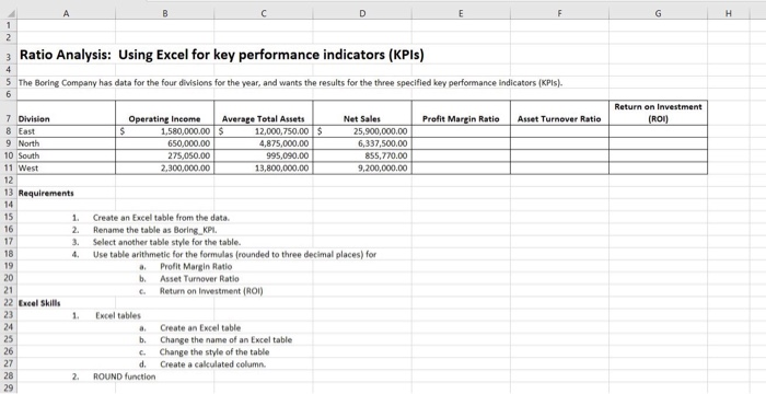
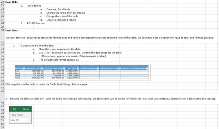
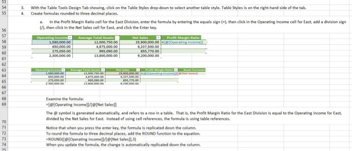
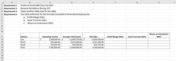
3 Ratio Analysis: Using Excel for key performance indicators (KPIs) 5 The Boring Company has data for the four divisions for the year, and wants the results for the three specified key performance Indicators (KPIs). Return on Investment Profit Margin Ratio Asset Turnover Ratio (ROI $ 7 Division 8 East 9 North 10 South 11 West Operating Income 1.580,000.00 650,000.00 225.050.00 2,300,000.00 Average Total Assets $ 12.000.750.00 4,875,000.00 995.090.00 13,800,000.00 Net Sales 25.900.000,00 6,337,500.00 855.720.00 9,200,000.00 13 Requirements 15 16 1. 2. 3. 4. Create an Excel table from the data Rename the table as Boring KPI. Select another table style for the table. Use table arithmetic for the formulas (rounded to three decimal places) for a. Profit Margin Ratio b, Asset Turnover Ratio c. Return on Investment (ROI) 19 21 22 Eucal Skills 1. Excel tables . b. C. d. ROUND function Create an Excel table Change the name of an Excel table Change the style of the table Create a cakulated column. 2. 22 Excel Skills 1. 26 Excel tables a. b. C. d. ROUND function Create an Excel table Change the name of an Excel table Change the style of the table Create a calculated column. 27 2. 30 Excel Hints An Excel table will allow you to create the formula once and have it automatically replicate down the rows of the table. An Excel table has a header row, rows of data, and formula columns. 1. To create a table from the data: a. Place the cursor anywhere in the data. b. Use CTRL-T to convert data to a table. Confirm the data range for the table. (Alternatively, you can use Insert > Table to create a table.) C. The default table format appears as 38 39 Operating Incom Pront Margin Anturnover Meturn Average Total Aise Net Sales 12.000.750 0 25,00,000.00 4,879.000.000.137.500.00 99.000. 00 ,77000 41 42 43 Click anywhere in the table to cause the Table Tools Design Tab to appear. 2. Rename the table as Solar_KPI. With the Table Tools Design Tab showing the table name will be on the left-hand side. You must use contiguous characters for a table name (no spaces). He Home Table Name 3. 4. With the Table Tools Design Tab showing, click on the Table Styles drop-down to select another table style. Table Styles is on the right-hand side of the tab. Create formulas rounded to three decimal places. a. in the Profit Margin Ratio cell for the East Division, enter the formula by entering the equals sign (=), then click in the Operating Income cell for East, add a division sign 1. then click in the Net Sales cell for East, and click the Enter key, Profit Margin Ratio Operating Incomell 650 000.00 275.050.00 2.300,000.00 4,375,000.00 995,000.00 13,000,000.00 Net Sales 25,900,000.00 6.137.500.00 155, 770.00 9,200,000.00 e r rage letals Come 25.000.000.00 855.770.00 Examine the formula: -@[Operating Income VI@Net Sales)] The symbol is generated automatically, and refers to a row in a table. That is, the Profit Margin Ratio for the East Division is equal to the Operating income for East, divided by the Net Sales for East. Instead of using cell references, the formula is using table references. Notice that when you press the enter key, the formula is replicated down the column. To round the formula to three decimal places, add the ROUND function to the equation ROUNDIT Operating Income Net Sales]1.3) When you update the formula, the change is automatically replicated down the column 1 Requirement i 2 Requirement 2 3 Requirement 3 4 Requirement 4 Create an Excel table from the data. Rename the table as Boring KPI. Select another table style for the table Use table arithmetic for the formulas (rounded to three decimal places) for a. Profit Margin Ratio b. Asset Turnover Ratio c. Return on Investment (ROI) Return on Investment Division Profit Margin Ratio Asset Turnover Ratio ROW $ Operating Income 1.580,000.00 650,000.00 225,050.00 2,300,000.00 Average Total Assets $ 12,000,750.00 4,875,000.00 995,090.00 13,800,000.00 Net Sales 25.900,000.00 6,337,500.00 855.770.00 9,200,000.00 South West
