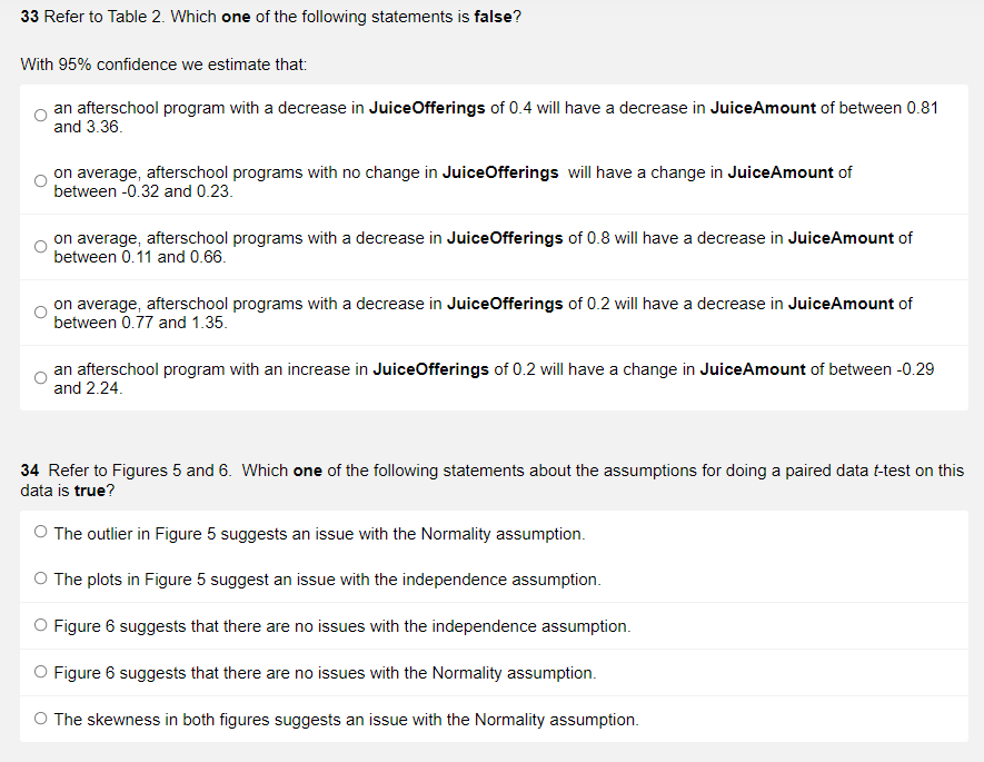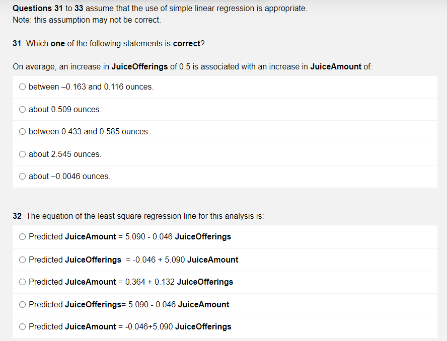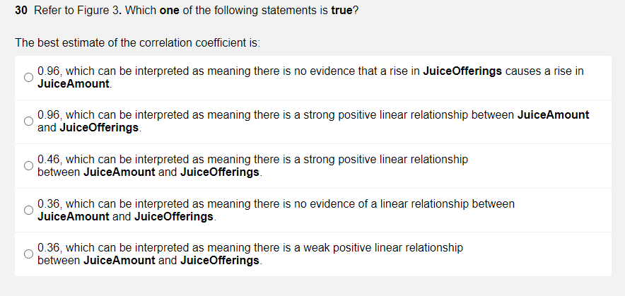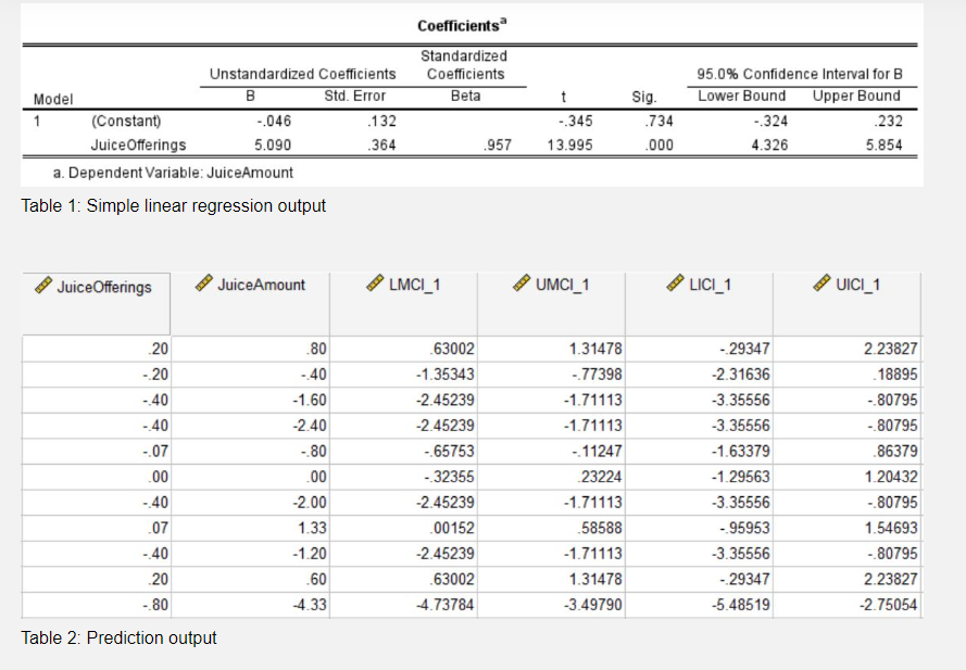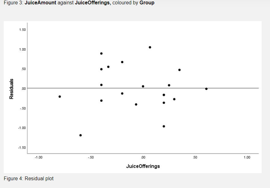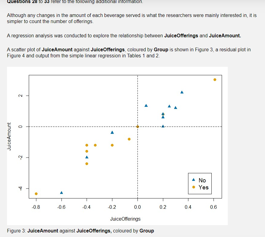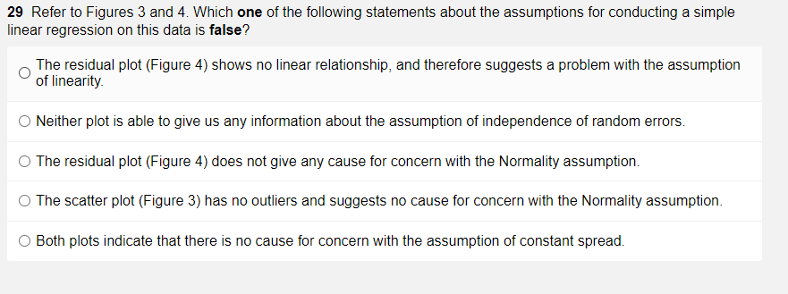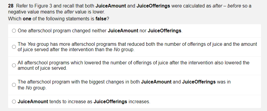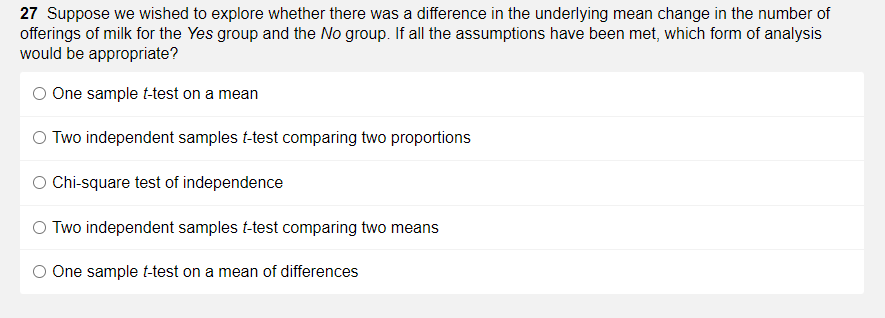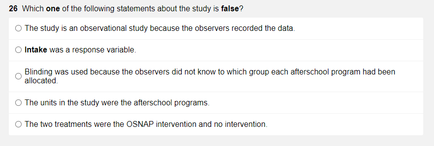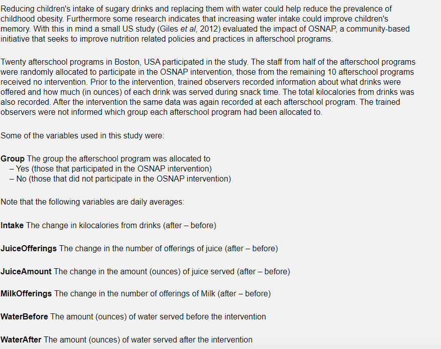
33 Refer to Table 2. Which one of the following statements is false? With 95% confidence we estimate that: an afterschool program with a decrease in Juice Offerings of 0.4 will have a decrease in JuiceAmount of between 0.81 and 3.36. on average, afterschool programs with no change in JuiceOfferings will have a change in JuiceAmount of between -0.32 and 0.23. on average, afterschool programs with a decrease in Juice Offerings of 0.8 will have a decrease in JuiceAmount of between 0.11 and 0.66. on average, afterschool programs with a decrease in JuiceOfferings of 0.2 will have a decrease in JuiceAmount of between 0.77 and 1.35. an afterschool program with an increase in JuiceOfferings of 0.2 will have a change in JuiceAmount of between -0.29 and 2.24. 34 Refer to Figures 5 and 6. Which one of the following statements about the assumptions for doing a paired data t-test on this data is true? O The outlier in Figure 5 suggests an issue with the Normality assumption. O The plots in Figure 5 suggest an issue with the independence assumption. O Figure 6 suggests that there are no issues with the independence assumption. Figure 6 suggests that there are no issues with the Normality assumption. The skewness in both figures suggests an issue with the Normality assumption. Questions 31 to 33 assume that the use of simple linear regression is appropriate. Note: this assumption may not be correct. 31 Which one of the following statements is correct? On average, an increase in Juice Offerings of 0.5 is associated with an increase in JuiceAmount of: between -0.163 and 0.116 ounces. about 0.509 ounces. between 0.433 and 0.585 ounces. about 2.545 ounces. about -0.0046 ounces. 32 The equation of the least square regression line for this analysis is: O Predicted JuiceAmount = 5.090 -0.046 JuiceOfferings Predicted Juice Offerings = -0.046 +5.090 JuiceAmount Predicted JuiceAmount = 0.364 +0.132 JuiceOfferings Predicted Juice Offerings- 5.090 -0.046 JuiceAmount Predicted JuiceAmount = -0.046+5.090 JuiceOfferings 30 Refer to Figure 3. Which one of the following statements is true? The best estimate of the correlation coefficient is: 0.96, which can be interpreted as meaning there is no evidence that a rise in Juice Offerings causes a rise in JuiceAmount. 0.96, which can be interpreted as meaning there is a strong positive linear relationship between JuiceAmount and Juice Offerings. 0.46, which can be interpreted as meaning there is a strong positive linear relationship between JuiceAmount and JuiceOfferings. 0.36, which can be interpreted as meaning there is no evidence of a linear relationship between JuiceAmount and JuiceOfferings. 0.36, which can be interpreted as meaning there is a weak positive linear relationship between JuiceAmount and Juice Offerings. Unstandardized Coefficients Model B Std. Error 1 (Constant) -.046 Juice Offerings 5.090 a. Dependent Variable: JuiceAmount Table 1: Simple linear regression output Juice Offerings JuiceAmount GOOD 20 -20 -40 -40 -.07 .00 -40 .07 -40 20 -80 Table 2: Prediction output .80 -40 -1.60 -2.40 -.80 .00 -2.00 1.33 -1.20 .60 -4.33 .132 .364 Coefficients Standardized Coefficients Beta LMCI_1 63002 -1.35343 -2.45239 -2.45239 -.65753 -32355 -2.45239 00152 -2.45239 63002 -4.73784 t -.345 .957 13.995 UMCI_1 www. 1.31478 -.77398 -1.71113 -1.71113 -.11247 23224 -1.71113 58588 -1.71113 1.31478 -3.49790 Sig. .734 .000 95.0% Confidence Interval for B Lower Bound Upper Bound -.324 .232 4.326 5.854 LICI_1 -29347 -2.31636 -3.35556 -3.35556 -1.63379 -1.29563 -3.35556 -95953 -3.35556 -29347 -5.48519 UICI_1 2.23827 18895 -80795 -80795 86379 1.20432 -.80795 1.54693 -.80795 2.23827 -2.75054 Figure 3: JuiceAmount against JuiceOfferings, coloured by Group 1.50 1.00 50 .00 -.50 -1.00 -1.50 -1.00 .00 Juice Offerings Figure 4: Residual plot Residuals -.50 .50 1.00 Questions 28 to 33 refer to the following additional information. Although any changes in the amount of each beverage served is what the researchers were mainly interested in, it is simpler to count the number of offerings. A regression analysis was conducted to explore the relationship between JuiceOfferings and JuiceAmount. A scatter plot of JuiceAmount against Juice Offerings, coloured by Group is shown in Figure 3, a residual plot in Figure 4 and output from the simple linear regression in Tables 1 and 2. JuiceAmount 2 0 Y -0.8 -0.6 -0.4 -0.2 0.0 0.2 Juice Offerings Figure 3: JuiceAmount against JuiceOfferings, coloured by Group 0.4 No Yes 0.6 29 Refer to Figures 3 and 4. Which one of the following statements about the assumptions for conducting a simple linear regression on this data is false? The residual plot (Figure 4) shows no linear relationship, and therefore suggests a problem with the assumption of linearity. Neither plot is able to give us any information about the assumption of independence of random errors. The residual plot (Figure 4) does not give any cause for concern with the Normality assumption. The scatter plot (Figure 3) has no outliers and suggests no cause for concern with the Normality assumption. Both plots indicate that there is no cause for concern with the assumption of constant spread. 28 Refer to Figure 3 and recall that both JuiceAmount and JuiceOfferings were calculated as after - before so a negative value means the after value is lower. Which one of the following statements is false? O One afterschool program changed neither JuiceAmount nor Juice Offerings. The Yes group has more afterschool programs that reduced both the number of offerings of juice and the amount of juice served after the intervention than the No group. All afterschool programs which lowered the number of offerings of juice after the intervention also lowered the amount of juice served. The afterschool program with the biggest changes in both JuiceAmount and JuiceOfferings was in the No group. JuiceAmount tends to increase as JuiceOfferings increases. 27 Suppose we wished to explore whether there was a difference in the underlying mean change in the number of offerings of milk for the Yes group and the No group. If all the assumptions have been met, which form of analysis would be appropriate? O One sample t-test on a mean O Two independent samples t-test comparing two proportions Chi-square test of independence O Two independent samples t-test comparing two means O One sample t-test on a mean of differences 26 Which one of the following statements about the study is false? O The study is an observational study because the observers recorded the data. Intake was a response variable. Blinding was used because the observers did not know to which group each afterschool program had been allocated. O The units in the study were the afterschool programs. O The two treatments were the OSNAP intervention and no intervention. Reducing children's intake of sugary drinks and replacing them with water could help reduce the prevalence of childhood obesity. Furthermore some research indicates that increasing water intake could improve children's memory. With this in mind a small US study (Giles et al, 2012) evaluated the impact of OSNAP, a community-based initiative that seeks to improve nutrition related policies and practices in afterschool programs. Twenty afterschool programs in Boston, USA participated in the study. The staff from half of the afterschool programs were randomly allocated to participate in the OSNAP intervention, those from the remaining 10 afterschool programs received no intervention. Prior to the intervention, trained observers recorded information about what drinks were offered and how much (in ounces) of each drink was served during snack time. The total kilocalories from drinks was also recorded. After the intervention the same data was again recorded at each afterschool program. The trained observers were not informed which group each afterschool program had been allocated to. Some of the variables used in this study were: Group The group the afterschool program was allocated to - Yes (those that participated in the OSNAP intervention) - No (those that did not participate in the OSNAP intervention) Note that the following variables are daily averages: Intake The change in kilocalories from drinks (after - before) JuiceOfferings The change in the number of offerings of juice (after - before) JuiceAmount The change in the amount (ounces) of juice served (after - before) MilkOfferings The change in the number of offerings of Milk (after - before) WaterBefore The amount (ounces) of water served before the intervention WaterAfter The amount (ounces) of water served after the intervention 33 Refer to Table 2. Which one of the following statements is false? With 95% confidence we estimate that: an afterschool program with a decrease in Juice Offerings of 0.4 will have a decrease in JuiceAmount of between 0.81 and 3.36. on average, afterschool programs with no change in JuiceOfferings will have a change in JuiceAmount of between -0.32 and 0.23. on average, afterschool programs with a decrease in Juice Offerings of 0.8 will have a decrease in JuiceAmount of between 0.11 and 0.66. on average, afterschool programs with a decrease in JuiceOfferings of 0.2 will have a decrease in JuiceAmount of between 0.77 and 1.35. an afterschool program with an increase in JuiceOfferings of 0.2 will have a change in JuiceAmount of between -0.29 and 2.24. 34 Refer to Figures 5 and 6. Which one of the following statements about the assumptions for doing a paired data t-test on this data is true? O The outlier in Figure 5 suggests an issue with the Normality assumption. O The plots in Figure 5 suggest an issue with the independence assumption. O Figure 6 suggests that there are no issues with the independence assumption. Figure 6 suggests that there are no issues with the Normality assumption. The skewness in both figures suggests an issue with the Normality assumption. Questions 31 to 33 assume that the use of simple linear regression is appropriate. Note: this assumption may not be correct. 31 Which one of the following statements is correct? On average, an increase in Juice Offerings of 0.5 is associated with an increase in JuiceAmount of: between -0.163 and 0.116 ounces. about 0.509 ounces. between 0.433 and 0.585 ounces. about 2.545 ounces. about -0.0046 ounces. 32 The equation of the least square regression line for this analysis is: O Predicted JuiceAmount = 5.090 -0.046 JuiceOfferings Predicted Juice Offerings = -0.046 +5.090 JuiceAmount Predicted JuiceAmount = 0.364 +0.132 JuiceOfferings Predicted Juice Offerings- 5.090 -0.046 JuiceAmount Predicted JuiceAmount = -0.046+5.090 JuiceOfferings 30 Refer to Figure 3. Which one of the following statements is true? The best estimate of the correlation coefficient is: 0.96, which can be interpreted as meaning there is no evidence that a rise in Juice Offerings causes a rise in JuiceAmount. 0.96, which can be interpreted as meaning there is a strong positive linear relationship between JuiceAmount and Juice Offerings. 0.46, which can be interpreted as meaning there is a strong positive linear relationship between JuiceAmount and JuiceOfferings. 0.36, which can be interpreted as meaning there is no evidence of a linear relationship between JuiceAmount and JuiceOfferings. 0.36, which can be interpreted as meaning there is a weak positive linear relationship between JuiceAmount and Juice Offerings. Unstandardized Coefficients Model B Std. Error 1 (Constant) -.046 Juice Offerings 5.090 a. Dependent Variable: JuiceAmount Table 1: Simple linear regression output Juice Offerings JuiceAmount GOOD 20 -20 -40 -40 -.07 .00 -40 .07 -40 20 -80 Table 2: Prediction output .80 -40 -1.60 -2.40 -.80 .00 -2.00 1.33 -1.20 .60 -4.33 .132 .364 Coefficients Standardized Coefficients Beta LMCI_1 63002 -1.35343 -2.45239 -2.45239 -.65753 -32355 -2.45239 00152 -2.45239 63002 -4.73784 t -.345 .957 13.995 UMCI_1 www. 1.31478 -.77398 -1.71113 -1.71113 -.11247 23224 -1.71113 58588 -1.71113 1.31478 -3.49790 Sig. .734 .000 95.0% Confidence Interval for B Lower Bound Upper Bound -.324 .232 4.326 5.854 LICI_1 -29347 -2.31636 -3.35556 -3.35556 -1.63379 -1.29563 -3.35556 -95953 -3.35556 -29347 -5.48519 UICI_1 2.23827 18895 -80795 -80795 86379 1.20432 -.80795 1.54693 -.80795 2.23827 -2.75054 Figure 3: JuiceAmount against JuiceOfferings, coloured by Group 1.50 1.00 50 .00 -.50 -1.00 -1.50 -1.00 .00 Juice Offerings Figure 4: Residual plot Residuals -.50 .50 1.00 Questions 28 to 33 refer to the following additional information. Although any changes in the amount of each beverage served is what the researchers were mainly interested in, it is simpler to count the number of offerings. A regression analysis was conducted to explore the relationship between JuiceOfferings and JuiceAmount. A scatter plot of JuiceAmount against Juice Offerings, coloured by Group is shown in Figure 3, a residual plot in Figure 4 and output from the simple linear regression in Tables 1 and 2. JuiceAmount 2 0 Y -0.8 -0.6 -0.4 -0.2 0.0 0.2 Juice Offerings Figure 3: JuiceAmount against JuiceOfferings, coloured by Group 0.4 No Yes 0.6 29 Refer to Figures 3 and 4. Which one of the following statements about the assumptions for conducting a simple linear regression on this data is false? The residual plot (Figure 4) shows no linear relationship, and therefore suggests a problem with the assumption of linearity. Neither plot is able to give us any information about the assumption of independence of random errors. The residual plot (Figure 4) does not give any cause for concern with the Normality assumption. The scatter plot (Figure 3) has no outliers and suggests no cause for concern with the Normality assumption. Both plots indicate that there is no cause for concern with the assumption of constant spread. 28 Refer to Figure 3 and recall that both JuiceAmount and JuiceOfferings were calculated as after - before so a negative value means the after value is lower. Which one of the following statements is false? O One afterschool program changed neither JuiceAmount nor Juice Offerings. The Yes group has more afterschool programs that reduced both the number of offerings of juice and the amount of juice served after the intervention than the No group. All afterschool programs which lowered the number of offerings of juice after the intervention also lowered the amount of juice served. The afterschool program with the biggest changes in both JuiceAmount and JuiceOfferings was in the No group. JuiceAmount tends to increase as JuiceOfferings increases. 27 Suppose we wished to explore whether there was a difference in the underlying mean change in the number of offerings of milk for the Yes group and the No group. If all the assumptions have been met, which form of analysis would be appropriate? O One sample t-test on a mean O Two independent samples t-test comparing two proportions Chi-square test of independence O Two independent samples t-test comparing two means O One sample t-test on a mean of differences 26 Which one of the following statements about the study is false? O The study is an observational study because the observers recorded the data. Intake was a response variable. Blinding was used because the observers did not know to which group each afterschool program had been allocated. O The units in the study were the afterschool programs. O The two treatments were the OSNAP intervention and no intervention. Reducing children's intake of sugary drinks and replacing them with water could help reduce the prevalence of childhood obesity. Furthermore some research indicates that increasing water intake could improve children's memory. With this in mind a small US study (Giles et al, 2012) evaluated the impact of OSNAP, a community-based initiative that seeks to improve nutrition related policies and practices in afterschool programs. Twenty afterschool programs in Boston, USA participated in the study. The staff from half of the afterschool programs were randomly allocated to participate in the OSNAP intervention, those from the remaining 10 afterschool programs received no intervention. Prior to the intervention, trained observers recorded information about what drinks were offered and how much (in ounces) of each drink was served during snack time. The total kilocalories from drinks was also recorded. After the intervention the same data was again recorded at each afterschool program. The trained observers were not informed which group each afterschool program had been allocated to. Some of the variables used in this study were: Group The group the afterschool program was allocated to - Yes (those that participated in the OSNAP intervention) - No (those that did not participate in the OSNAP intervention) Note that the following variables are daily averages: Intake The change in kilocalories from drinks (after - before) JuiceOfferings The change in the number of offerings of juice (after - before) JuiceAmount The change in the amount (ounces) of juice served (after - before) MilkOfferings The change in the number of offerings of Milk (after - before) WaterBefore The amount (ounces) of water served before the intervention WaterAfter The amount (ounces) of water served after the intervention