

!
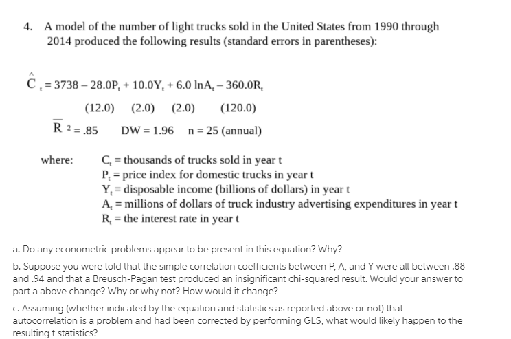
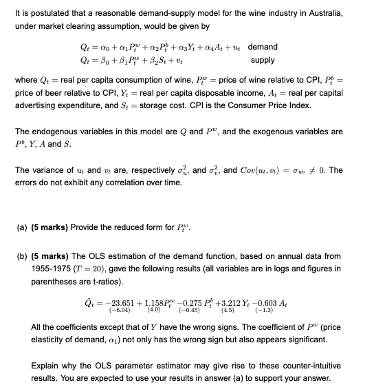
4. A model of the number of light trucks sold in the United States from 1990 through 2014 produced the following results (standard errors in parentheses): C , = 3738 - 28.0P, + 10.0Y, + 6.0 InA, - 360.0R. (12.0) (2.0) (2.0) (120.0) R 2 =.85 DW = 1.96 n = 25 (annual) where: C = thousands of trucks sold in year t P. = price index for domestic trucks in year t Y. = disposable income (billions of dollars) in year t A = millions of dollars of truck industry advertising expenditures in year t R = the interest rate in year t a. Do any econometric problems appear to be present in this equation? Why? b. Suppose you were told that the simple correlation coefficients between P, A, and Y were all between .88 and .94 and that a Breusch-Pagan test produced an insignificant chi-squared result. Would your answer to part a above change? Why or why not? How would it change? c. Assuming (whether indicated by the equation and statistics as reported above or not) that autocorrelation is a problem and had been corrected by performing GLS, what would likely happen to the resulting t statistics?It is postulated that a reasonable demand-supply model for the wine industry in Australia, under market clearing assumption, would be given by Qt = ontop" +azpi tash toA tu demand Qt = Po+ BIP"" + ByS + the supply where Q: = real per capita consumption of wine, Po = price of wine relative to CPI, Ph = price of beer relative to CPI, Y, = real per capita disposable income, A, = real per capital advertising expenditure, and S, = storage cost. CPI is the Consumer Price Index. The endogenous variables in this model are @ and P", and the exogenous variables are p, Y, A and S. The variance of wt and t are, respectively on, and of, and Cov(us, ") = Our # 0. The errors do not exhibit any correlation over time. (a) (5 marks) Provide the reduced form for Pu. (b) (5 marks) The OLS estimation of the demand function, based on annual data from 1955-1975 (7 = 20), gave the following results (all variables are in logs and figures in parentheses are t-ratios). Q+ = -23.651 + 1.158PM -0.275 P +3.212 Y, -0.603 At (-6.04) (4.0) (-0.45) (4.5) (-1.3) All the coefficients except that of Y have the wrong signs. The coefficient of P" (price elasticity of demand, o) not only has the wrong sign but also appears significant. Explain why the OLS parameter estimator may give rise to these counter-intuitive results. You are expected to use your results in answer (a) to support your answer.1. 1. Consider an economy that produces the single good"output" with two factors of production, land {T} and labor (L). The gure to the n'ght shows how the marginal product of labor varies with changes in the amount of labor employed. If this simple economy employs O G womers, its total output is given by and labor's total wages by 2. The gure to the right illustrates the causes and effects of international labor mobility between two countries, Home and Foreign {*1 The horizontal axis represents the total wond labor force. The workers employed in Home are measured from the left. the workers employed in Foreign from the right. The left vertical axis shows the marginal product of labor in Home; the right vertical axis shows the marginal product of labor in Foreign. Suppose the initial allocation of labor has [II L1 workers in Home and 0*L'l workers in Foreign. Given this initial allocation, labor can be expected to 3. The diagram to the n'ght depicts a country's production possibilities frontier before {TH} and after ('II'E}, a biased expansion of its production possibilities. If it is known that this shi occurred because of an increase in land supply, one can deduce that the landintensive good must be 4. The table below contains the unit labor requirements in Home and Foreign for each of ve goods as well as the relative productivity advantage of Home. Assume there are no transportation costs. Fill in the ve blanks in the table below. {Enter your responses rounded to one decimal place where necessary.) Given the data in the preceding table, we know that 'rfthe relative Home wage (wiv) = 1 QS 8-4 Units-of-production depreciation LO P1 On January 2, 2015, the Matthews Band acquires sound equipment for concert performances at a cost of $65,800. The band estimates it will use this equipment for four years, during which time it anticipates performing about 200 concerts. It estimates that after four years it can sell the equipment for $2,000. During year 2015, the band performs 45 concerts. Compute the year 2015 depreciation using the units-of-production method. Select formula for the depreciation rate of Units of Production: Calculate 2015 depreciation expense: Depreciation per concert Concerts in 2015 Depreciation in 2015Rizio Co. purchases a machine for $12,500, terms 2/10, n/60, FOB shipping point. The seller prepaid the $360 freight charges, adding the amount to the invoice and bringing its total to $12,860. The machine requires special steel mounting and power connections costing $895. Another $475 is paid to assemble the machine and get it into operation. In moving the machine to its steel mounting, $180 in damages occurred. Materials costing $40 are used in adjusting the machine to produce a satisfactory product. The adjustments are normal for this machine and are not the result of the damages. Complete the below table to calculate the cost recorded for this machine. (Rizio pays for this machine within the cash discount period.) Amount Included in Cost of Equipment: Invoice price of machine Net purchase price Total cost to be recordedA researcher has data on class size (CS) and average test scores from 100 econometrics classes (TS). He estimates the OLS regression and obtains the following regression line: TS = 520.4-5.82 x CS reg (20.4) (2.21) where the R2 = 0.08, SER = 11.5, and the standard errors of each coefficient is in parentheses underneath. inf a) What are Bo and B1, and what are their standard errors? 51 b) Interpret the R for this regression. c) A classroom has 22 students. What is the regression's prediction for that classroom's average test score? d) Last year a classroom had 19 students and this year it has 23 students. What is the regression's prediction for the change in the classroom average test score? (Hint: A change of 1 unit of X induces a change of B 1 units in Y, so a change in 4 units of X will induce what change in Y?) e) The sample average class size across the 100 classrooms is 21.4. What is the sample average of test scores across the 100 classrooms? (Hint: The estimated regression line (above) gives you the average relationship between Y and X!) f) Is Bi significant at the 5% significance level (i.e. can you reject the null that B 1 = 0)? (Hint: Same procedure as 4b where the critical value is now for 98 degrees of freedom at the 5% level-see Table 2) . g) Construct a 95% confidence interval for 1, the regression slope coefficient.3. An economics department at a large state university keeps track of its majors' starting salaries. Does taking econometrics affect starting salary? Let SAL = salary in dollars, GPA = grade point average on a 4.0 scale, METRICS = 1 if student took econometrics, and METRICS = 0 otherwise. Using the data file metrics.dat, which contains information on 50 recent graduates, we obtain the estimated regression SAL = 24200 + 1643GPA + 5033METRICS R= = 0.74 (se ) (1078) (352) (456) (a) Interpret the estimated equation. (b) How would you modify the equation to see whether women had lower starting salaries than men? (Hint: Define an indicator variable FEMALE = 1, if female; zero otherwise.) (c) How would you modify the equation to see if the value of econometrics was the same for men and women


