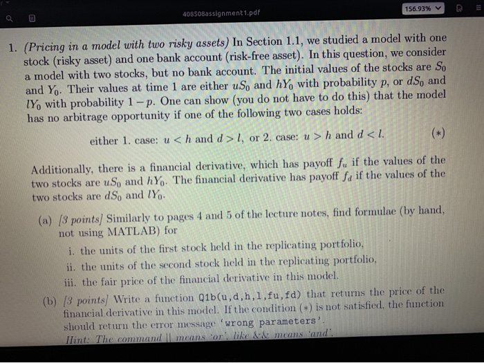
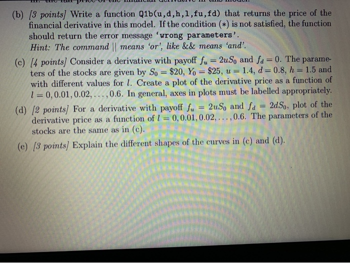
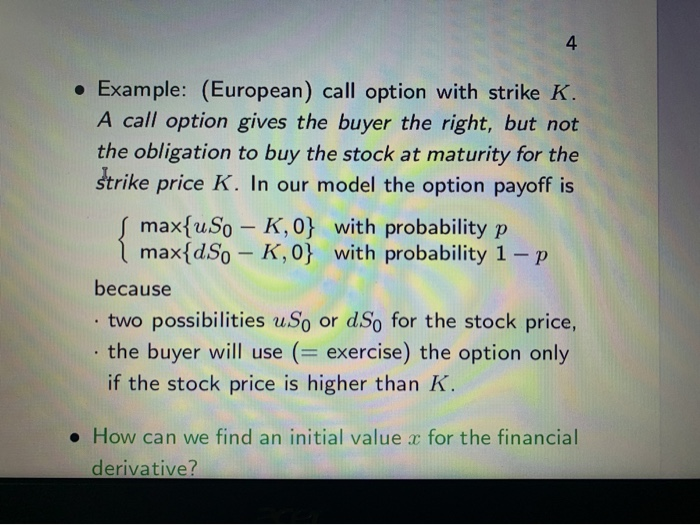
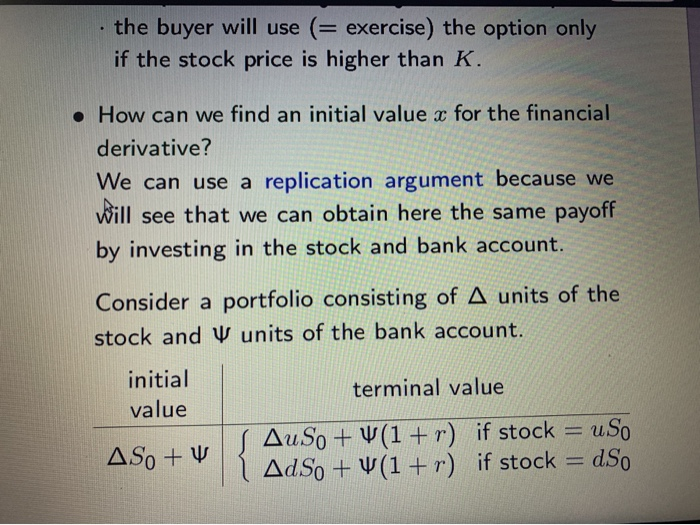
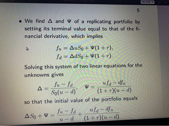
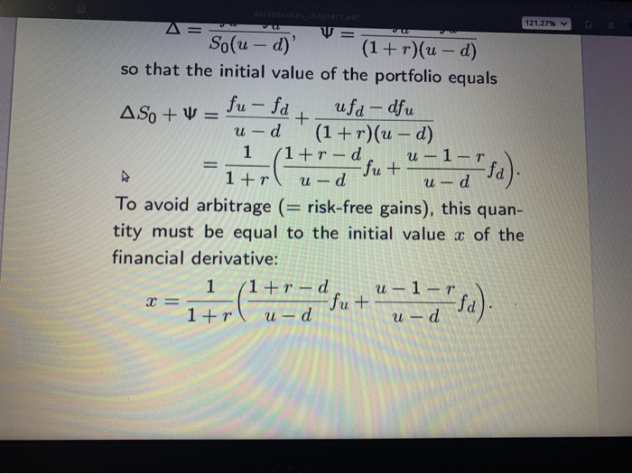
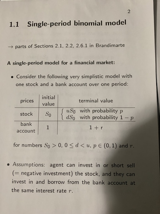
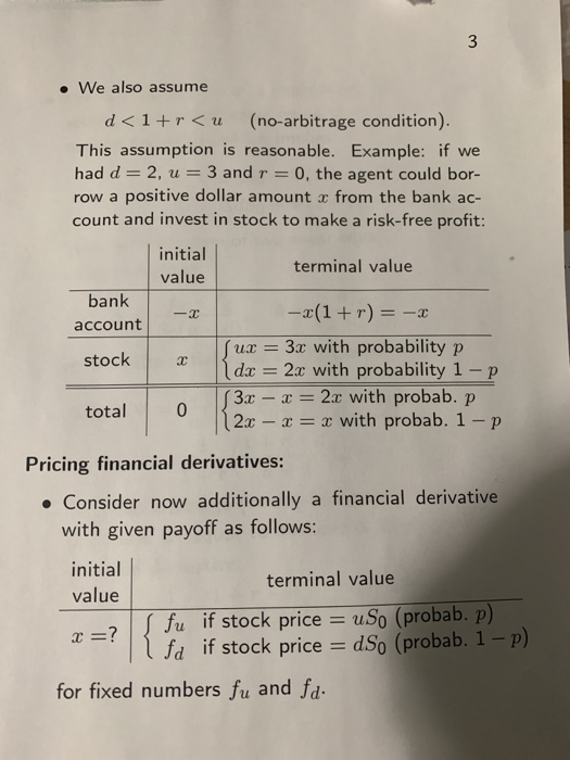
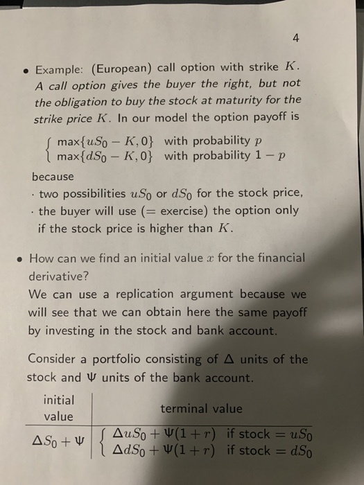
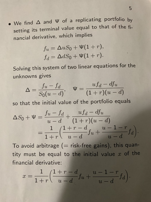
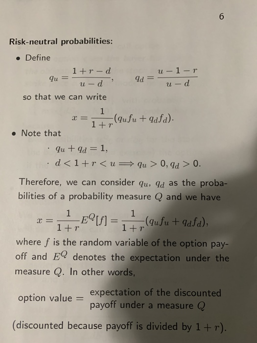
408508assignment 1.pdf 156,93% 1. (Pricing in a model with two risky assets) In Section 1.1, we studied a model with one stock (risky asset) and one bank account (risk-free asset). In this question, we consider a model with two stocks, but no bank account. The initial values of the stocks are So and Y. Their values at time 1 are either uso and hy, with probability p, or ds, and IY, with probability 1-p. One can show (you do not have to do this, that the model has no arbitrage opportunity if one of the following two cases holds: either 1. case: u 1, or 2. case: u >h and d 0, 0 0,9d > 0. 1+T Therefore, we can consider quId as the proba- bilities of a probability measure Q and we have 1 1 * = 12,5[f] = 1, (qufu + qafa), where f is the random variable of the option pay- off and EQ denotes the expectation under the measure Q. In other words, _expectation of the discounted option value = payoff under a measure Q (discounted because payoff is divided by 1+r). A crucial observation is that the probability mea- sure Q used in the pricing formula does not equal the historical (from the model construction) prob- ability measure because in general it r- d u -1-r. - u-d 1+1 +p, qu =- qd= 1 - 1 -d 41- p. 250 + 4d1+1 . If we calculate the expectation of the discounted stock price under Q, we obtain Lofterminal value of stock 1tr uso do + 1+T 1+1 1+r-duso u-1-r dSo u-d 1tr u-d 1tr = So, which shows that the expectation of the discounted terminal stock price under Q equals its initial value. Therefore, qu and qd are called risk-neutral prob- abilities and Q a risk-neutral probability measure. 408508assignment 1.pdf 156,93% 1. (Pricing in a model with two risky assets) In Section 1.1, we studied a model with one stock (risky asset) and one bank account (risk-free asset). In this question, we consider a model with two stocks, but no bank account. The initial values of the stocks are So and Y. Their values at time 1 are either uso and hy, with probability p, or ds, and IY, with probability 1-p. One can show (you do not have to do this, that the model has no arbitrage opportunity if one of the following two cases holds: either 1. case: u 1, or 2. case: u >h and d 0, 0 0,9d > 0. 1+T Therefore, we can consider quId as the proba- bilities of a probability measure Q and we have 1 1 * = 12,5[f] = 1, (qufu + qafa), where f is the random variable of the option pay- off and EQ denotes the expectation under the measure Q. In other words, _expectation of the discounted option value = payoff under a measure Q (discounted because payoff is divided by 1+r). A crucial observation is that the probability mea- sure Q used in the pricing formula does not equal the historical (from the model construction) prob- ability measure because in general it r- d u -1-r. - u-d 1+1 +p, qu =- qd= 1 - 1 -d 41- p. 250 + 4d1+1 . If we calculate the expectation of the discounted stock price under Q, we obtain Lofterminal value of stock 1tr uso do + 1+T 1+1 1+r-duso u-1-r dSo u-d 1tr u-d 1tr = So, which shows that the expectation of the discounted terminal stock price under Q equals its initial value. Therefore, qu and qd are called risk-neutral prob- abilities and Q a risk-neutral probability measure