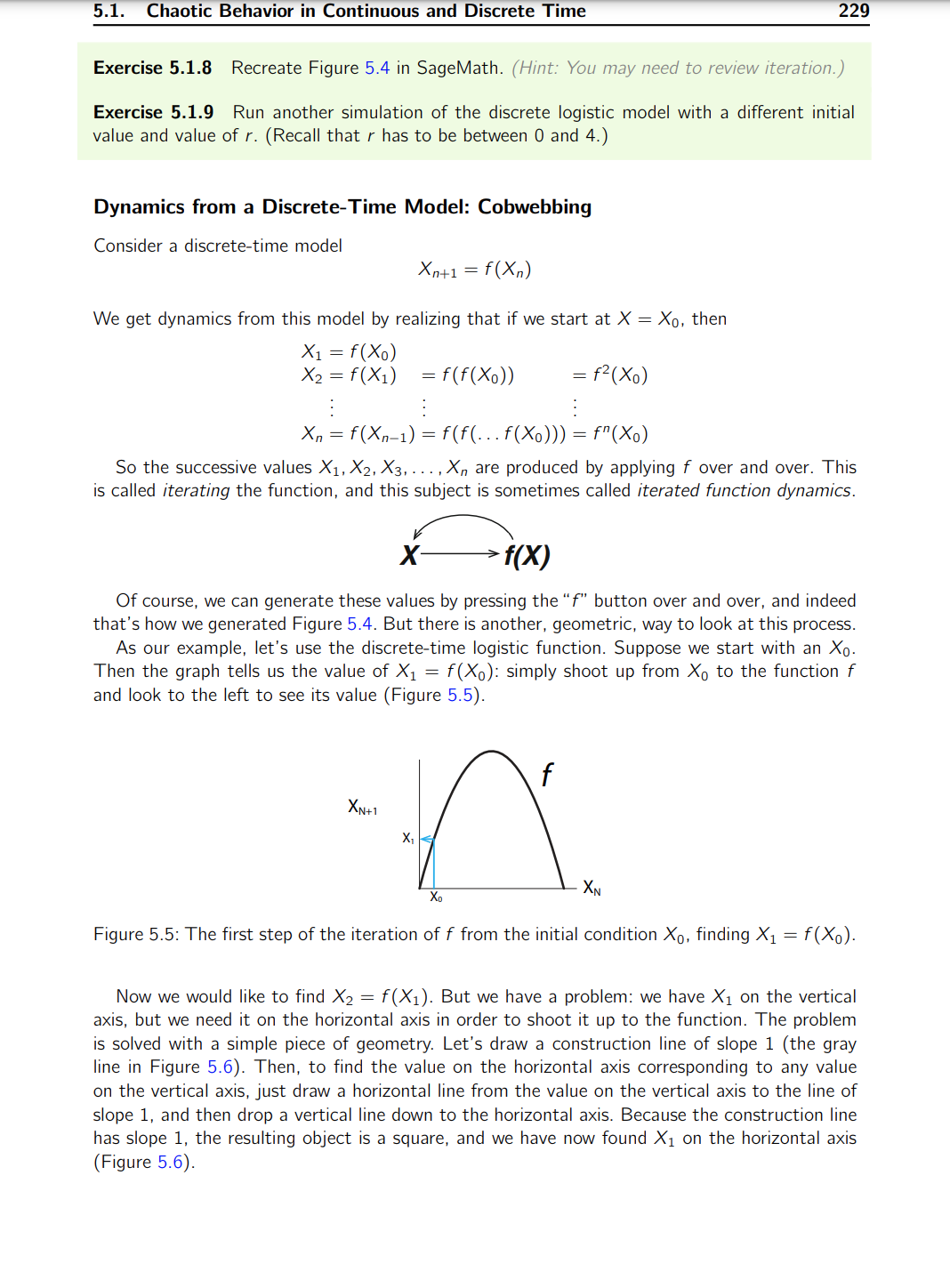
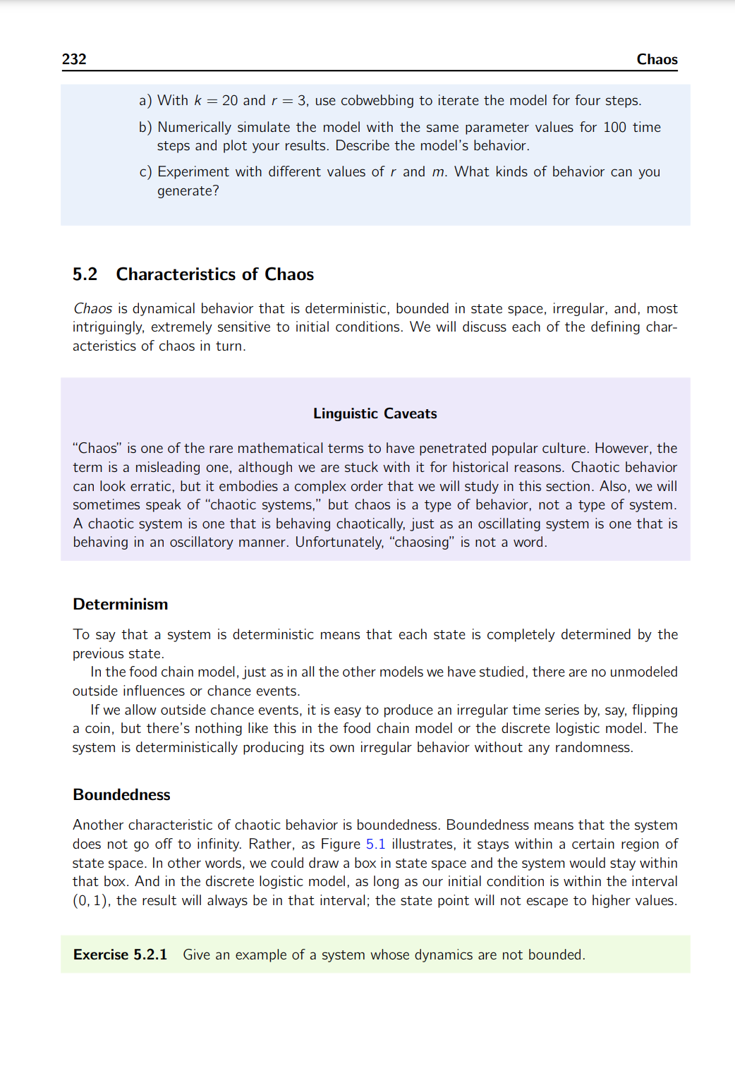
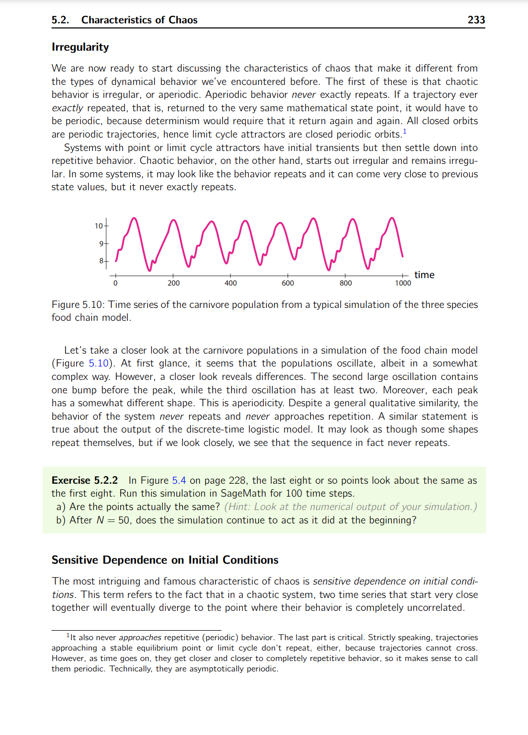
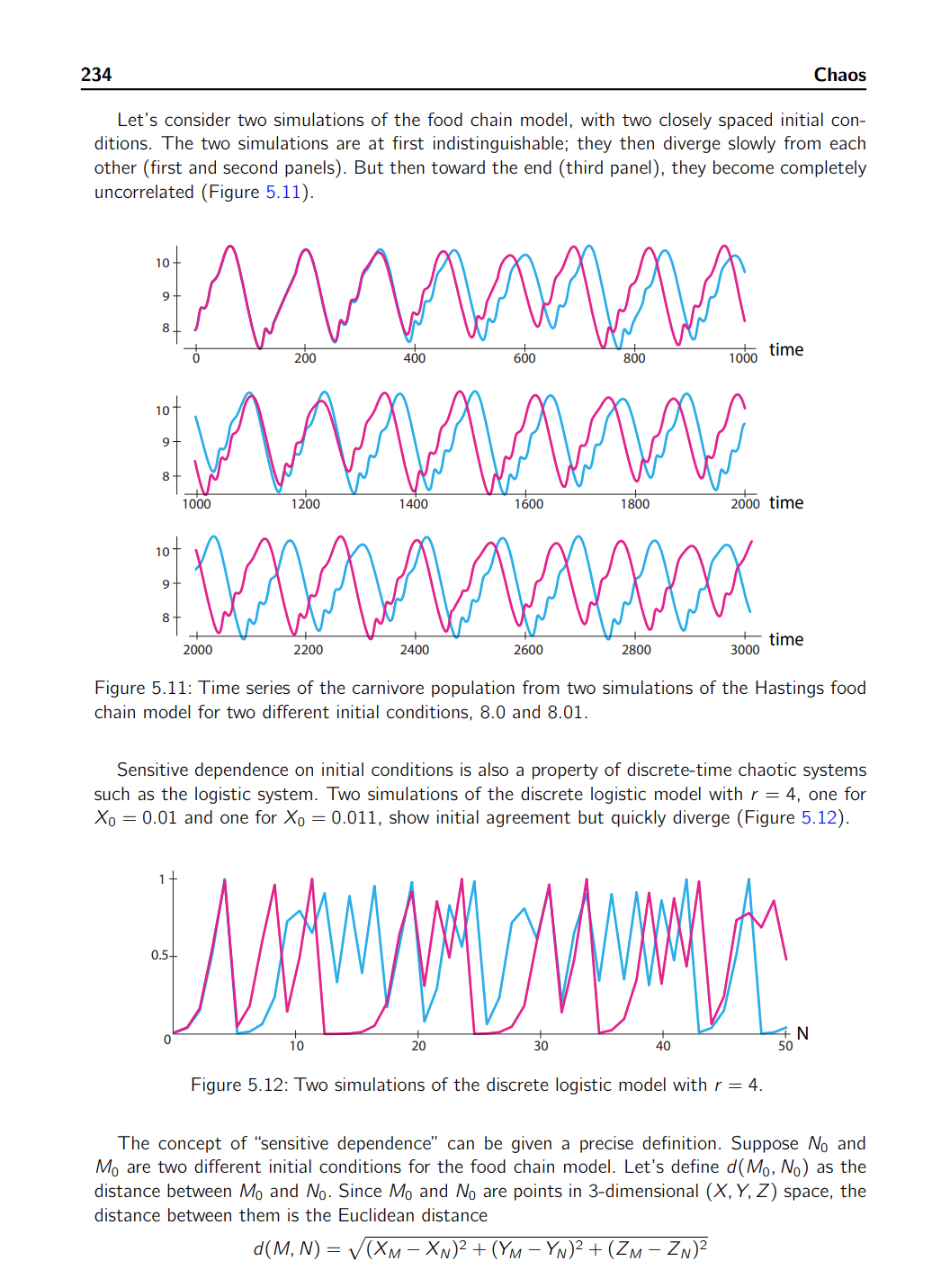
5.1. Chaotic Behavior in Continuous and Discrete Time 225 is different from one cycle to the next, as is the exact shape of each cycle. So the output is not really periodic. It appears to be somewhat periodic, but also to have some kind of randomness. If we consider a 3D trajectory generated by the model. we see a complex shape that does not resemble the simple points and loops we've seen before. It looks like an upside-down jug. The path of a typical state point begins in the jug part and then spirals inward mostly in the X-Y plane. while slowly rising along the Z axis. Finally. the state point gets thrown into the handle of thejug. where it plummets down to begin another cycle. The nonrepeating time series and associated complex trajectories are hallmarks of the dynamical behavior known as chaos (Figure 5.1). Exercise 5.1.1 Simulate the food chain model in SageMath for at least two sets of initial conditions. Plot the results as both time series and trajectories. (For the latter. you can use zip to combine three lists of values before plotting them with listiplot .) Use the parameter values given in the caption of Figure 5.1. In order to understand chaotic behavior. we will first introduce a different kind of dynamical model. one in which time advances in discrete steps. After learning what we need to there. we will come back to differential equations and continuous time. Discrete-Time Dynamical Systems In a discrete-time model. time advances in discrete steps. In differential equations. time is the continuous variable t. But in a discretetime system. time comes in discrete intervals 0. 1. 2. 3. . . . . with no values between them. Therefore. we represent \"time" by the integer-valued variable N. so N=O.1.2.3..... Such models work well for organisms with well-defined breeding seasons or in other situations in which the data come at discrete times. For example. heartbeats are discrete; there are the Nth heartbeat and the (N + 1)st heartbeat. but nothing in between. Consider a deer population growing at 5% a year. If population size is denoted by the variable X. its value at time N is written X(N) or XN (pronounced \"X of N"). Then, we can write an equation that gives us XN+1 as a function of XN. X...+1 : X... + 0.05x... : 10st (52) This kind of equation, which gives the population size at time N+ 1 in terms ofthat at time N. is called a difference equation. The value 1.05 in equation (5.2) is typically represented by the parameter r. so the general difference equation is XN+1 = I'XN (5.3) When r > 1. the population is growing. and when r 1, representing growth, r can be less than 1, representing a quantity that decreases over time. The trait-fife of a radioactive element is the amount of time needed for half the element to decay. What traction of the initial amount of such an element will remain after ten half-lives? Exercise 5.1.6 When money in a bank account accrues compound interest. the interest earned in one time period is added to the principal, and then the sum is used as the base for the next time period. a) If you start off with $1000 and earn 2% interest that is compounded annually. how much money will you have in 5 years? In 10 years? In 20 years? b) How long will it take you to accumulate $10,000? The Discrete-Time Logistic Model We will now develop and examine an important discrete-time model, the discrete logistic equation (May 1976). Consider a population of insects that live one year, lay eggs, and then die. The insect popu- lation in year N + 1 is a function of the population in year N. If we call the population X, then XN+1 = XN). Suppose there are enough resources to support a maximum of K insects. It the current population is XN, then the current population is using only 5,} of the total resources available. But that means that the fraction of total resources that are unused is 1 %. it is these unused resources that are available to support new births. Therefore, just as in the continuous-time logistic equation model, we will assume that the per capita insect birth rate is proportional to the available resources. with proportionality constant r. This gives us X per capita birth rateN : r(1 7 YN) As always, the per capita birth rate must be multiplied by the population size XN to get the XN total birth rate. Then the population as a whole lays rXN( T) eggs in year N, and since no adults survive from one year to the next, and assuming that each egg laid leads to a mature adult that reproduces, XN XN+1 = FXNil * 7) This equation has two parameters, r and K. To simplify our analysis of its behavior, we can set K : 1, so the numbers XN can be interpreted as fractions of the carrying capacity. We then 228 Chaos have the equation XN+1= {XN(1XN) (5.4) Exercise 5.1.7 if r : 1.2 and X0 : 0.42. what is X1? X2? Equation (5.4) is called the discrete logistic equation or the discrete logistic model. As usual, \"discrete" refers to time (Figure 5.3). The state of the system can be any number between 0 and l. The discrete logistic model isjust as deterministic as all the other models we've studied. There is no randomness in equation (5.4). Also, we specified that the maximum possible insect population is 1, and as long as r S 4. the population will indeed stay between 0 and 1. Thus, the dynamics of this system are bounded. Simulating this model (using iteration) gives us a surprisingly irregular time series (Figure 5.4). 0.8 0.6 XN+I 0.4 0.2 0 0.2 0.4 0.5 0.3 1XN Figure 5.3: Graph of the function XN+1 : rXN(1 7 XN) for r : 4. While this time series is irregular, there are also some predictable aspects to the behavior. Note. for example. that when the state variable takes values close to zero, the subsequent changes are small. Similarly, when the state variable takes values near 0.75. the subsequent changes are also small (look around N : 10 and N : 2?). We will see why shortly. Figure 5.4: A simulation of the discrete logistic model with r : 4 and X0 : 0.01. 5.1. Chaotic Behavior in Continuous and Discrete Time 229 Exercise 5.1.3 Recreate Figure 5.4 in Sagelvlath. {Hint You may need to rowers .'TCi-Li'fi'OH Exercise 5.1.9 Run another simulation of the discrete logistic model with a different initial value and value of r. (Recall that r has to be between 0 and 4.) Dynamics from a Discrete-Time Model: Cobwebbing Consider a discrete-time model Xn+1 = f(xii) We get dynamics from this model by realizing that if we start at X : X0. then x1 : axe) X2 : mm 2 WWW) = f2(Xo) x. '= mm) '= \"1% . . axe) '= f\"(Xo) So the successive values X1.X2. X3 ..... X\" are produced by applying 1' over and over. This is called iterating the function. and this subject is sometimes called iterated function dynamics. x> f(X) Of course. we can generate these values by pressing the \"1'" button over and over. and indeed that's how we generated Figure 5.4. But there is another. geometric. way to look at this process. As our example. let's use the discrete-time logistic function. Suppose we start with an X0. Then the graph tells us the value of X1 = f(Xo): simply shoot up from X0 to the function f and look to the left to see its value (Figure 5.5). Xu Figure 5.5: The first step of the iteration of 1' from the initial condition X0. finding X1 : {(XO). Now we would like to find X2 : f(X1). But we have a problem: we have X1 on the vertical axis. but we need it on the horizontal axis in order to shoot it up to the function. The problem is solved with a simple piece of geometry. Let's draw a construction line of slope 1 (the gray line in Figure 5.6). Then. to find the value on the horizontal axis corresponding to any value on the vertical axis. just draw a horizontal line from the value on the vertical axis to the line of slope 1. and then drop a vertical line down to the horizontal axis. Because the construction line has slope 1. the resulting object is a square. and we have now found X1 on the horizontal axis (Figure 5.6). 232 Chaos a) With k : 20 and r : 3, use cobwebbing to iterate the model for four steps. b) Numerically simulate the model with the same parameter values for 100 time steps and plot your results. Describe the model's behavior. c) Experiment with different values of r and m. What kinds of behavior can you generate? 5.2 Characteristics of Chaos Chaos is dynamical behavior that is deterministic, bounded in state space, irregular. and. most intriguingly, extremely sensitive to initial conditions. We will discuss each of the defining char- acteristics of chaos in turn. Linguistic Caveats \"Chaos" is one of the rare mathematical terms to have penetrated popular culture. However. the term is a misleading one, although we are stuck with it for historical reasons. Chaotic behavior can look erratic. but it embodies a complex order that we will study in this section. Also. we will sometimes speak of \"chaotic systems." but chaos is a type of behavior, not a type of system. A chaotic system is one that is behaving chaotically, just as an oscillating system is one that is behaving in an oscillatory manner. Unfortunately. "chaosing" is not a word. Determinism To say that a system is deterministic means that each state is completely determined by the previous state. In the food chain model,just as in all the other models we have studied, there are no unmodeled outside influences or chance events. If we allow outside chance events. it is easy to produce an irregular time series by. say, flipping a coin, but there's nothing like this in the food chain model or the discrete logistic model. The system is deterministically producing its own irregular behavior without any randomness. Boundedness Another characteristic of chaotic behavior is boundedness. Boundedness means that the system does not go off to infinity. Rather, as Figure 5.] illustrates, it stays within a certain region of state space. In other words. we could draw a box in state space and the system would stay within that box. And in the discrete logistic model, as long as our initial condition is within the interval (0.1), the result will always be in that interval; the state point will not escape to higher values. Exercise 5.2.1 Give an example of a system whose dynamics are not bounded. 5.2. Characteristics of Chaos 233 Irregularity We are now ready to start discussing the characteristics of chaos that make it different from the types of dynamical behavior we've encountered before. The first of these is that chaotic behavior is irregular, or aperiodic. Aperiodic behavior never exactly repeats. If a trajectory ever exactly repeated, that is. returned to the very same mathematical state point. it would have to be periodic. because determinism would require that it return again and again. All closed orbits are periodic trajectories. hence limit cycle attractors are closed periodic orbits.1 Systems with point or limit cycle attractors have initial transients but then settle down into repetitive behavior. Chaotic behavior, on the other hand. starts out irregular and remains irreg u- lar. In some systems. it may look like the behavior repeats and it can come very close to previous state values. but it never exactly repeats. 10 . I . I i time 0 200 400 500 BOD 'l 000 Figure 5.10: Time series of the carnivore population from a typical simulation ofthe three species food chain model. Let's take a closer look at the carnivore populations in a simulation of the food chain model (Figure 5.10). At first glance. it seems that the populations oscillate, albeit in a somewhat complex way. However. a closer look reveals differences. The second large oscillation contains one bump before the peak. while the third oscillation has at least two. Moreover. each peak has a somewhat different shape. This is aperiodicity. Despite a general qualitative similarity. the behavior of the system never repeats and never approaches repetition. A similar statement is true about the output of the discrete-time logistic model. It may look as though some shapes repeat themselves. but if we look closely, we see that the sequence in fact never repeats. Exercise 5.2.2 In Figure 5.4 on page 228. the last eight or so points look about the same as the first eight. Run this simulation in SageMath for 100 time steps. a) Are the points actually the same? (Hint Look at the numerical output at vow S.-'.'iiii:'iff0f7 j b) After N : 50. does the simulation continue to act as it did at the beginning? Sensitive Dependence an Initial Conditions The most intriguing and famous characteristic of chaos is sensitive dependence on initiai condi- tions. This term refers to the fact that in a chaotic system. two time series that start very close together will eventually diverge to the point where their behavior is completely uncorrelated. 1It also never approaches repetitive (periodic) behavior. The last part is critical. Strictly speaking' trajectories approaching a stable equilibrium point or limit cycle don't repeat. either, because trayectories cannot cross. However. as time goes on. they get closer and closer to completely repetitive behavior, so it makes sense to call them periodic. Technically. they are asymptotically periodic. 234 Chaos Let's consider two simulations of the food chain model, with two closely spaced initial con- ditions. The two simulations are at first indistinguishable: they then diverge slowly from each other (first and second panels). But then toward the end (third panel), they become completely uncorrelated (Figure 5.11). 10 9 - B 2, l) 200 400 500 000 who time 10 2 9 __ e _ 1000 i 200 1400 1600 1300 2000 time 1D ' 9 _ B _ 2000 2200 2400 2500 2000 3000 time Figure 5.11: Time series of the carnivore population from two simulations of the Hastings food chain model for two different initial conditions. 8.0 and 8.01. Sensitive dependence on initial conditions is also a property of discrete-time chaotic systems such as the logistic system. Two simulations of the discrete logistic model with r = 4. one for X0 : 0.01 and one for X0 : 0.011. show initial agreement but quickly diverge (Figure 5.12). Figure 5112: Two simulations of the discrete logistic model with r : 4. The concept of "sensitive dependence" can be given a precise definition. Suppose N0 and MD are two different initial conditions for the food chain model. Let's define d(Mo, NO) as the distance between M0 and N9. Since MD and N0 are points in 3dimensional (X, Y, Z) space. the distance between them is the Euclidean distance dW'. N) = \\/(XM - X0)2 + (W - YNF + [Z0 - ZN)2