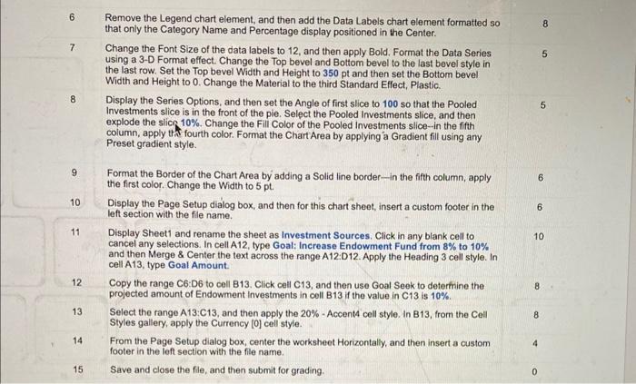
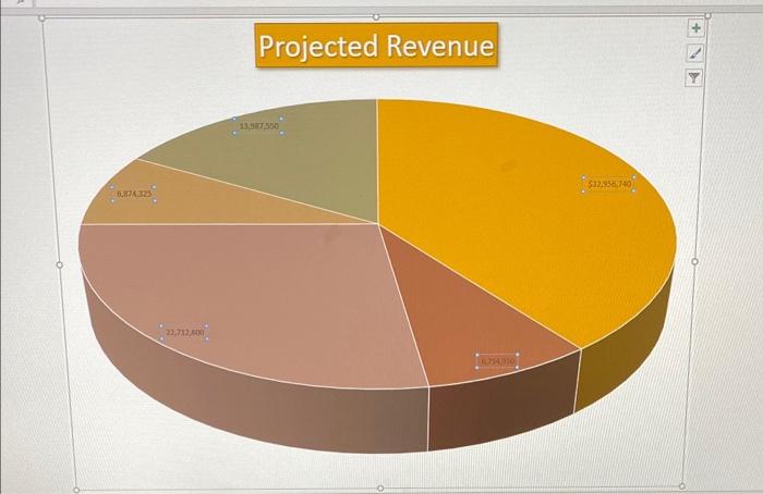
6 7 8 6 10 10 11 Remove the Legend chart element, and then add the Data Labels chart element formatted so that only the Category Name and Percentage display positioned in the Center. Change the Font Size of the data labels to 12, and then apply Bold. Format the Data Series using a 3-D Format effect. Change the Top bevel and Bottom bevel to the last bevel style in the last row. Set the Top bevel Width and Height to 350 pt and then set the Bottom bevel Width and Height to 0. Change the Material to the third Standard Effect, Plastic. Display the Series Options, and then set the Angle of first slice to 100 so that the Pooled Investments slice is in the front of the pie. Select the Pooled Investments slice, and then explode the slice 10%. Change the Fill Color of the Pooled Investments slice--in the fifth column, apply the fourth color. Format the Chart Area by applying a Gradient fill using any Preset gradient style. Format the Border of the Chart Area by adding a Solid line border-in the fifth column, apply the first color. Change the Width to 5 pt. Display the Page Setup dialog box, and then for this chart sheet, insert a custom footer in the left section with the file name. Display Sheet1 and rename the sheet as Investment Sources. Click in any blank cell to cancel any selections. In cell A12, type Goal: Increase Endowment Fund from 8% to 10% and then Merge & Center the text across the range A12:D12. Apply the Heading 3 cell style. In cell A13, type Goal Amount. 8 5 5 6 6 10 12 12 Copy the range C6:D6 to cell B13. Click cell C13, and then use Goal Seek to determine the projected amount of Endowment Investments in cell B13 if the value in C13 is 10%. 8 13 Select the range A13:C13, and then apply the 20% - Accent4 cell style. In B13, from the Cell Styles gallery, apply the Currency [0] cell style. 8 14 From the Page Setup dialog box, center the worksheet Horizontally, and then insert a custom footer in the left section with the file name. 4 15 Save and close the file, and then submit for grading.