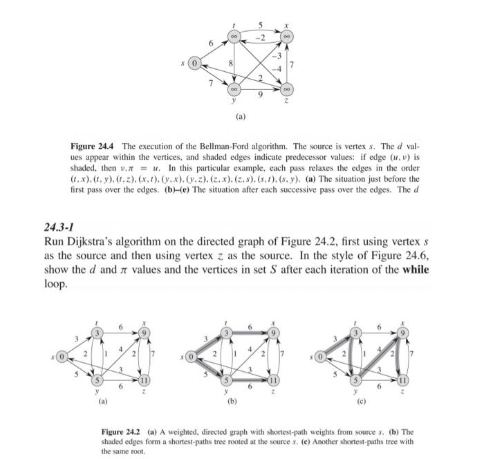
. 6 oc 4 7 00 9 Figure 24.4 The execution of the Bellman-Ford algorithm. The source is vertex s. The d val- ues appear within the vertices, and shaded edges indicate predecessor values: if edge (u.v) is shaded, then v. = u. In this particular example, each pass relaxes the edges in the order (1x). (.y).(4.2).(x,1),(,x),(v.).(.x). (z.s). (s.1).(sy). (a) The situation just before the first pass over the edges. (b)-(e) The situation after each successive pass over the edges. The d 24.3-1 Run Dijkstra's algorithm on the directed graph of Figure 24.2, first using vertex s as the source and then using vertex z as the source. In the style of Figure 24.6, show the d and a values and the vertices in set S after each iteration of the while loop. 4 N 2 y Figure 24.2 (a) A weighted, directed graph with shortest-path weights from sources. (b) The shaded edges form a shortest-paths tree rooted at the sources. (c) Another shortest-paths tree with the same root . 6 oc 4 7 00 9 Figure 24.4 The execution of the Bellman-Ford algorithm. The source is vertex s. The d val- ues appear within the vertices, and shaded edges indicate predecessor values: if edge (u.v) is shaded, then v. = u. In this particular example, each pass relaxes the edges in the order (1x). (.y).(4.2).(x,1),(,x),(v.).(.x). (z.s). (s.1).(sy). (a) The situation just before the first pass over the edges. (b)-(e) The situation after each successive pass over the edges. The d 24.3-1 Run Dijkstra's algorithm on the directed graph of Figure 24.2, first using vertex s as the source and then using vertex z as the source. In the style of Figure 24.6, show the d and a values and the vertices in set S after each iteration of the while loop. 4 N 2 y Figure 24.2 (a) A weighted, directed graph with shortest-path weights from sources. (b) The shaded edges form a shortest-paths tree rooted at the sources. (c) Another shortest-paths tree with the same root