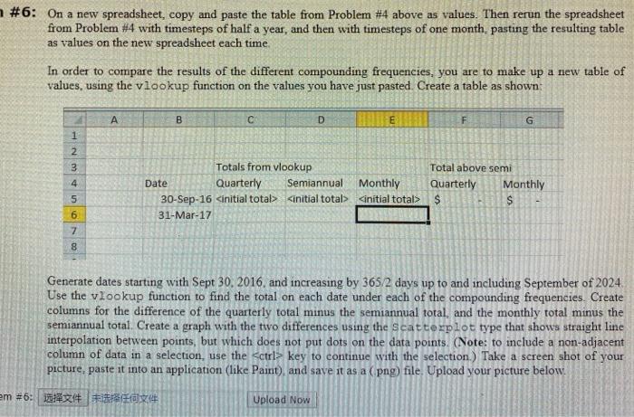
#6: On a new spreadsheet, copy and paste the table from Problem #4 above as values. Then rerun the spreadsheet from Problem #4 with timesteps of half a year, and then with timesteps of one month, pasting the resulting table as values on the new spreadsheet each time In order to compare the results of the different compounding frequencies, you are to make up a new table of values, using the vlookup function on the values you have just pasted Create a table as shown: A B D F G 3 4 5 . 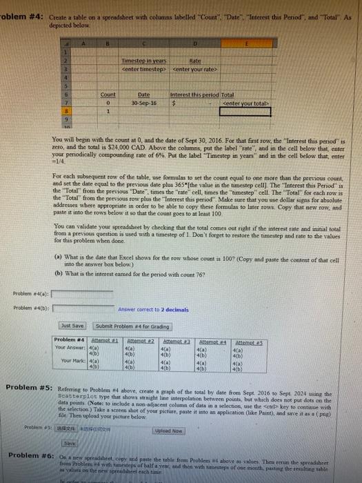Totals from vlookup Total above semi Date Quarterly Semiannual Monthly Quarterly Monthly 30-Sep-16 key to continue with the selection.) Take a screen shot of your picture, paste it into an application (like Paint), and save it as a (png) file Upload your picture below. em #6: Tit kim (4) C# Upload Now oblem #4: Create a table on a spreadsheet with columns labelled "Count", "Date" "Interest this period", and "Total" As depicted below. A B D 1 Timestep in years center timestep Rate Center your rates 4 5 Count 0 7 Date 30-Sep-16 Interest this period Total $ center your total 1 9 You will begin with the count at 0, and the date of Sept 30, 2016. For that first row, the "Interest this periodis zero, and the total is $24,000 CAD. Above the columns, put the label "rate", and in the cell below that, enter your periodically compounding rate of 6% Put the label "Timestep in years and in the cell below that, enter 1/4 For each subsequent row of the table, use formulas to set the count equal to one more than the previous count, and set the date equal to the previous date plus 365"(the value in the timestep cell] The "Interest this periods the "Total from the previous "Date", times the "rate" cell, times the "tumestep" cell. The "Total for each row is the "Total from the previous row plus the Interest this period" Make sure that you use dollar signs for absolute addresses where appropriate in order to be able to copy these formulas to later rows. Copy that new row, and paste it into the rows below it so that the count goes to at least 100 You can validate your spreadsheet by checking that the total comes out right of the interest rate and initial total from a previous question is used with a timestep of 1. Don't forget to restore the timestep and rate to the values for this problem when done. (a) What is the date that Excel shows for the row whose count is 100? (Copy and paste the content of that cell into the answer box below) (b) What is the interest earned for the period with count 76? Problem 4(a): Problem 4(1): Answer correct to 2 decimals Just Save Submit Problem for Grading Attempts Problem 4 Attemat Your Answer: 4(a) (b) Your Market 4) 4/6) Att 2 4a) 4(b) 4(a) Atomta 4a) 4[b) 4(a) 4(b) Attemet 4(a) 4(b) 410) 4b) 460) 4a) 4(b Problem #5: Reming to Problem above, create a graph of the total by date from Sept. 2016 10 Sept 2021 wsing the Scatterplot type that shows straight line interpolation between points, but which does not put dots on the data points (Note: to include a non adjacent column of data in a selection, use the ctrl key to continue with the selection) Take a screen shot of your picture, paste it into an application like Paint), and save it as a file. This upload your picture below Problem: Upload Now Dav Problem #6: Onew prese, copy and paste the table from Problem above as values. The rerun the spreadsheet from Problem with me eps of half a year and then with timesteps of one month to the reste table on the new read each time #6: On a new spreadsheet, copy and paste the table from Problem #4 above as values. Then rerun the spreadsheet from Problem #4 with timesteps of half a year, and then with timesteps of one month, pasting the resulting table as values on the new spreadsheet each time In order to compare the results of the different compounding frequencies, you are to make up a new table of values, using the vlookup function on the values you have just pasted Create a table as shown: A B D F G 3 4 5 . Totals from vlookup Total above semi Date Quarterly Semiannual Monthly Quarterly Monthly 30-Sep-16 key to continue with the selection.) Take a screen shot of your picture, paste it into an application (like Paint), and save it as a (png) file Upload your picture below. em #6: Tit kim (4) C# Upload Now oblem #4: Create a table on a spreadsheet with columns labelled "Count", "Date" "Interest this period", and "Total" As depicted below. A B D 1 Timestep in years center timestep Rate Center your rates 4 5 Count 0 7 Date 30-Sep-16 Interest this period Total $ center your total 1 9 You will begin with the count at 0, and the date of Sept 30, 2016. For that first row, the "Interest this periodis zero, and the total is $24,000 CAD. Above the columns, put the label "rate", and in the cell below that, enter your periodically compounding rate of 6% Put the label "Timestep in years and in the cell below that, enter 1/4 For each subsequent row of the table, use formulas to set the count equal to one more than the previous count, and set the date equal to the previous date plus 365"(the value in the timestep cell] The "Interest this periods the "Total from the previous "Date", times the "rate" cell, times the "tumestep" cell. The "Total for each row is the "Total from the previous row plus the Interest this period" Make sure that you use dollar signs for absolute addresses where appropriate in order to be able to copy these formulas to later rows. Copy that new row, and paste it into the rows below it so that the count goes to at least 100 You can validate your spreadsheet by checking that the total comes out right of the interest rate and initial total from a previous question is used with a timestep of 1. Don't forget to restore the timestep and rate to the values for this problem when done. (a) What is the date that Excel shows for the row whose count is 100? (Copy and paste the content of that cell into the answer box below) (b) What is the interest earned for the period with count 76? Problem 4(a): Problem 4(1): Answer correct to 2 decimals Just Save Submit Problem for Grading Attempts Problem 4 Attemat Your Answer: 4(a) (b) Your Market 4) 4/6) Att 2 4a) 4(b) 4(a) Atomta 4a) 4[b) 4(a) 4(b) Attemet 4(a) 4(b) 410) 4b) 460) 4a) 4(b Problem #5: Reming to Problem above, create a graph of the total by date from Sept. 2016 10 Sept 2021 wsing the Scatterplot type that shows straight line interpolation between points, but which does not put dots on the data points (Note: to include a non adjacent column of data in a selection, use the ctrl key to continue with the selection) Take a screen shot of your picture, paste it into an application like Paint), and save it as a file. This upload your picture below Problem: Upload Now Dav Problem #6: Onew prese, copy and paste the table from Problem above as values. The rerun the spreadsheet from Problem with me eps of half a year and then with timesteps of one month to the reste table on the new read each time