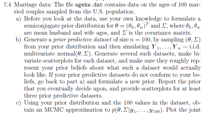
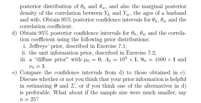
7.4 Marriage data: The file agehw . dat contains data on the ages of 100 mar- ried couples sampled from the U.S. population. a) Before you look at the data, use your own knowledge to formulate a semiconjugate prior distribution for 0 = (Oh, 0w)and E, where Oh, Qu are mean husband and wife ages, and _ is the covariance matrix. b) Generate a prior predictive dataset of size n = 100, by sampling (0, E) from your prior distribution and then simulating Y1, ..., Yn ~ i.i.d. multivariate normal(0, _). Generate several such datasets, make bi- variate scatterplots for each dataset, and make sure they roughly rep- resent your prior beliefs about what such a dataset would actually look like. If your prior predictive datasets do not conform to your be- liefs, go back to part a) and formulate a new prior. Report the prior that you eventually decide upon, and provide scatterplots for at least three prior predictive datasets. c) Using your prior distribution and the 100 values in the dataset, ob- tain an MCMC approximation to p(0, Ely1, . .., /100). Plot the jointposterior distribution of Oh and Ow, and also the marginal posterior density of the correlation between Yo and Yw, the ages of a husband and wife. Obtain 95% posterior confidence intervals for Oh, Ow and the correlation coefficient. d) Obtain 95% posterior confidence intervals for Oh, Ow and the correla- tion coefficient using the following prior distributions: i. Jeffreys' prior, described in Exercise 7.1; ii. the unit information prior, described in Exercise 7.2; iii. a "diffuse prior" with #o = 0, Ao = 105 x I, So = 1000 x I and Vo = 3. e) Compare the confidence intervals from d) to those obtained in c). Discuss whether or not you think that your prior information is helpful in estimating 0 and _, or if you think one of the alternatives in d) is preferable. What about if the sample size were much smaller, say n = 25