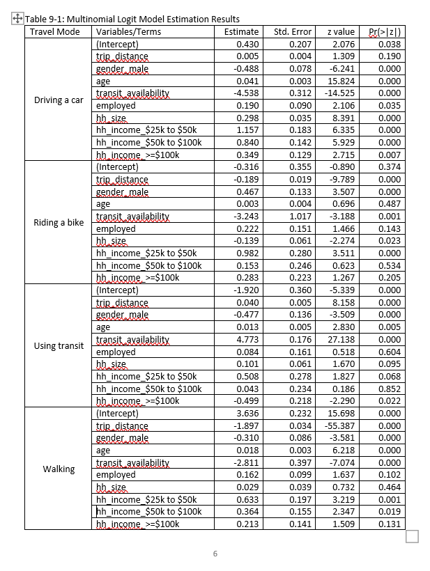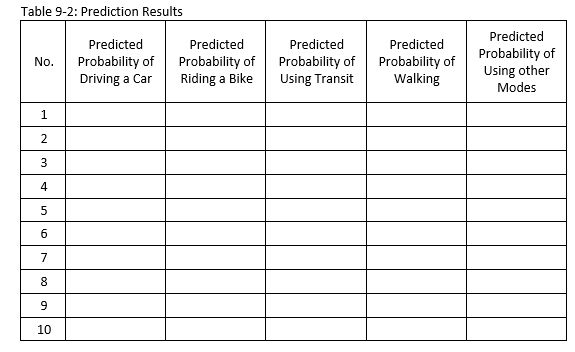
8. (15 points) According to the same survey data, we have developed a multinomial logit model to show the relationships between the mode choice and associated factors. The model considers five possible modes: car, bike, transit, walk and other. Table 9-1 shows the model estimation results. Use the model estimation results to predict the mode choice for 10 trips in attached spreadsheet (the same table for Question 7). Please have your predictions for each mode in Table 9-2. Table 9-1: Multinomial Logit Model Estimation Results Travel Mode Variables/Terms Estimate (Intercept) 0.430 trip.distance 0.005 gendermale -0.488 age 0.041 transit availability -4.538 Driving a car employed 0.190 hb size 0.298 hh_income_$25k to $50k 1.157 hh_income_$50k to $100k 0.840 hb income >=$100k 0.349 (Intercept) -0.316 trir distance -0.189 gender male 0.467 age 0.003 -3.243 transit availability Riding a bike employed 0.222 bh size -0.139 hh_income_$25k to $50k 0.982 hh_income_$50k to $100k 0.153 hb income >=$100k 0.283 (Intercept) -1.920 trip.distance 0.040 gender, male -0.477 age 0.013 4.773 transit availability Using transit employed 0.084 bh size 0.101 hh_income_$25k to $50k 0.508 hh income $50k to $100k 0.043 hh income >=$100k -0.499 (Intercept) 3.636 trip.distance -1.897 gender,male -0.310 age 0.018 transit availability -2.811 Walking employed 0.162 hh size 0.029 hh income_$25k to $50k 0.633 hh_income_$50k to $100k 0.364 hb income >=$100k 0.213 Std. Error 0.207 0.004 0.078 0.003 0.312 0.090 0.035 0.183 0.142 0.129 0.355 0.019 0.133 0.004 1.017 0.151 0.061 0.280 0.246 0.223 0.360 0.005 0.136 0.005 0.176 0.161 0.061 0.278 0.234 0.218 0.232 0.034 0.086 0.003 0.397 0.099 0.039 0.197 0.155 0.141 z value 2.076 1.309 -6.241 15.824 -14.525 2.106 8.391 6.335 5.929 2.715 -0.890 -9.789 3.507 0.696 -3.188 1.466 -2.274 3.511 0.623 1.267 -5.339 8.158 -3.509 2.830 27.138 0.518 1.670 1.827 0.186 -2.290 15.698 -55.387 -3.581 6.218 -7.074 1.637 0.732 3.219 2.347 1.509 Pr>[21) 0.038 0.190 0.000 0.000 0.000 0.035 0.000 0.000 0.000 0.007 0.374 0.000 0.000 0.487 0.001 0.143 0.023 0.000 0.534 0.205 0.000 0.000 0.000 0.005 0.000 0.604 0.095 0.068 0.852 0.022 0.000 0.000 0.000 0.000 0.000 0.102 0.464 0.001 0.019 0.131 6 Table 9-2: Prediction Results No. Predicted Probability of Driving a Car Predicted Probability of Riding a Bike Predicted Probability of Using Transit Predicted Probability of Walking Predicted Probability of Using other Modes 1 2 3 3 4 5 6 7 8 9 10 B D E| F G H | J K L M No. trip_distance gender male age transit_availability employed hh_size hh_income 100k 1 1 1 37 1 1 0 0 2 3 2 3 2 0 34 0 0 2.967 3.793 20.409 11.051 1 1 1 0 0 39 1 1 0 0 Nm 700 1 3 4 1 1 1 1 1 3 1 0 0 1 0 6 | 0000001 0 5 0 51 32 38 0 1 0 male female female male female male male female female male 0.918 15.063 1 >=$100k >=$100k $25k to $50k >=$100k $25k to $50k >=$100k $50k to $100k $25k to $50k $50k to $100k >=$100k 6 1 0 1 2 0 0 1 7 19.468 1 63 0 1 2 0 0 0 8 9 8 0 0 35 1 0 1 0 10 2.574 5.154 10.094 1 1 2 9 0 0 0 0 0 29 1 0 0 1 0 11 10 1 61 1 2 0 0 0 1 8. (15 points) According to the same survey data, we have developed a multinomial logit model to show the relationships between the mode choice and associated factors. The model considers five possible modes: car, bike, transit, walk and other. Table 9-1 shows the model estimation results. Use the model estimation results to predict the mode choice for 10 trips in attached spreadsheet (the same table for Question 7). Please have your predictions for each mode in Table 9-2. Table 9-1: Multinomial Logit Model Estimation Results Travel Mode Variables/Terms Estimate (Intercept) 0.430 trip.distance 0.005 gendermale -0.488 age 0.041 transit availability -4.538 Driving a car employed 0.190 hb size 0.298 hh_income_$25k to $50k 1.157 hh_income_$50k to $100k 0.840 hb income >=$100k 0.349 (Intercept) -0.316 trir distance -0.189 gender male 0.467 age 0.003 -3.243 transit availability Riding a bike employed 0.222 bh size -0.139 hh_income_$25k to $50k 0.982 hh_income_$50k to $100k 0.153 hb income >=$100k 0.283 (Intercept) -1.920 trip.distance 0.040 gender, male -0.477 age 0.013 4.773 transit availability Using transit employed 0.084 bh size 0.101 hh_income_$25k to $50k 0.508 hh income $50k to $100k 0.043 hh income >=$100k -0.499 (Intercept) 3.636 trip.distance -1.897 gender,male -0.310 age 0.018 transit availability -2.811 Walking employed 0.162 hh size 0.029 hh income_$25k to $50k 0.633 hh_income_$50k to $100k 0.364 hb income >=$100k 0.213 Std. Error 0.207 0.004 0.078 0.003 0.312 0.090 0.035 0.183 0.142 0.129 0.355 0.019 0.133 0.004 1.017 0.151 0.061 0.280 0.246 0.223 0.360 0.005 0.136 0.005 0.176 0.161 0.061 0.278 0.234 0.218 0.232 0.034 0.086 0.003 0.397 0.099 0.039 0.197 0.155 0.141 z value 2.076 1.309 -6.241 15.824 -14.525 2.106 8.391 6.335 5.929 2.715 -0.890 -9.789 3.507 0.696 -3.188 1.466 -2.274 3.511 0.623 1.267 -5.339 8.158 -3.509 2.830 27.138 0.518 1.670 1.827 0.186 -2.290 15.698 -55.387 -3.581 6.218 -7.074 1.637 0.732 3.219 2.347 1.509 Pr>[21) 0.038 0.190 0.000 0.000 0.000 0.035 0.000 0.000 0.000 0.007 0.374 0.000 0.000 0.487 0.001 0.143 0.023 0.000 0.534 0.205 0.000 0.000 0.000 0.005 0.000 0.604 0.095 0.068 0.852 0.022 0.000 0.000 0.000 0.000 0.000 0.102 0.464 0.001 0.019 0.131 6 Table 9-2: Prediction Results No. Predicted Probability of Driving a Car Predicted Probability of Riding a Bike Predicted Probability of Using Transit Predicted Probability of Walking Predicted Probability of Using other Modes 1 2 3 3 4 5 6 7 8 9 10 B D E| F G H | J K L M No. trip_distance gender male age transit_availability employed hh_size hh_income 100k 1 1 1 37 1 1 0 0 2 3 2 3 2 0 34 0 0 2.967 3.793 20.409 11.051 1 1 1 0 0 39 1 1 0 0 Nm 700 1 3 4 1 1 1 1 1 3 1 0 0 1 0 6 | 0000001 0 5 0 51 32 38 0 1 0 male female female male female male male female female male 0.918 15.063 1 >=$100k >=$100k $25k to $50k >=$100k $25k to $50k >=$100k $50k to $100k $25k to $50k $50k to $100k >=$100k 6 1 0 1 2 0 0 1 7 19.468 1 63 0 1 2 0 0 0 8 9 8 0 0 35 1 0 1 0 10 2.574 5.154 10.094 1 1 2 9 0 0 0 0 0 29 1 0 0 1 0 11 10 1 61 1 2 0 0 0 1