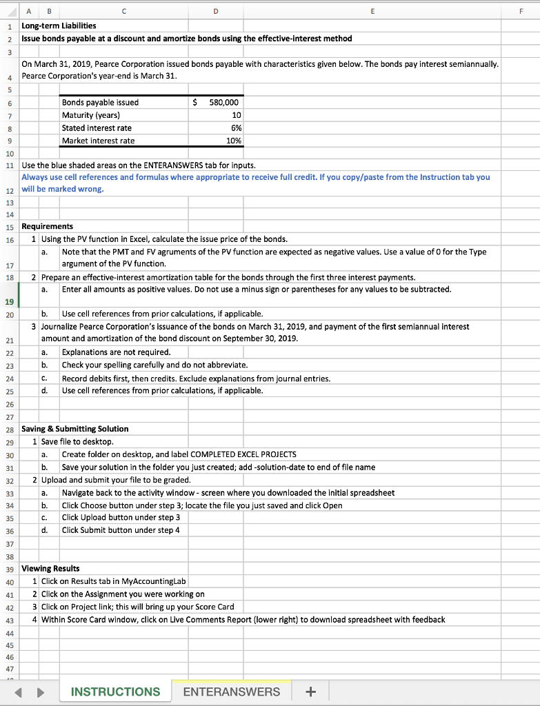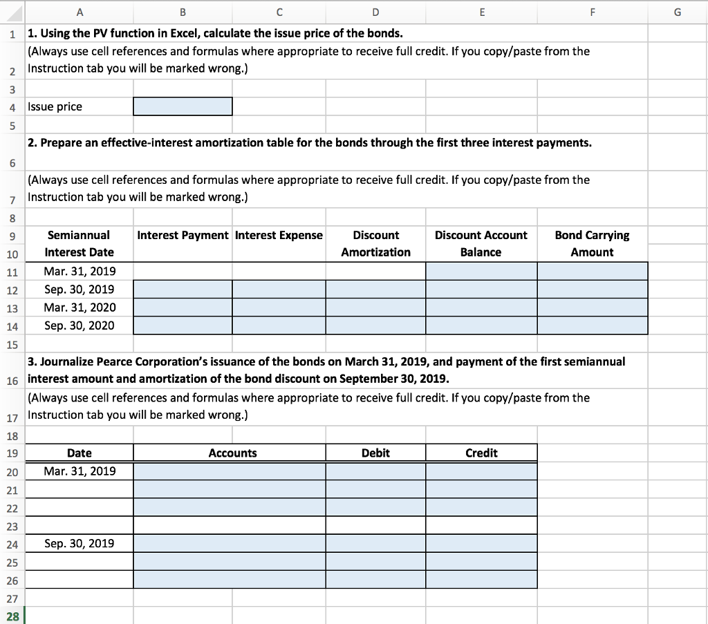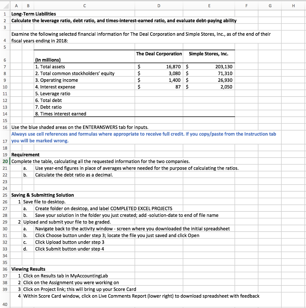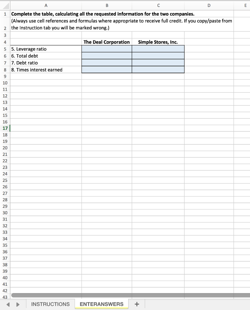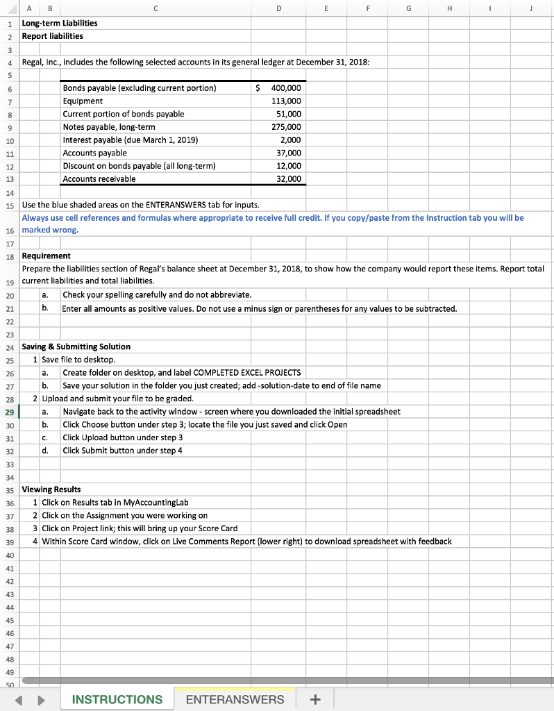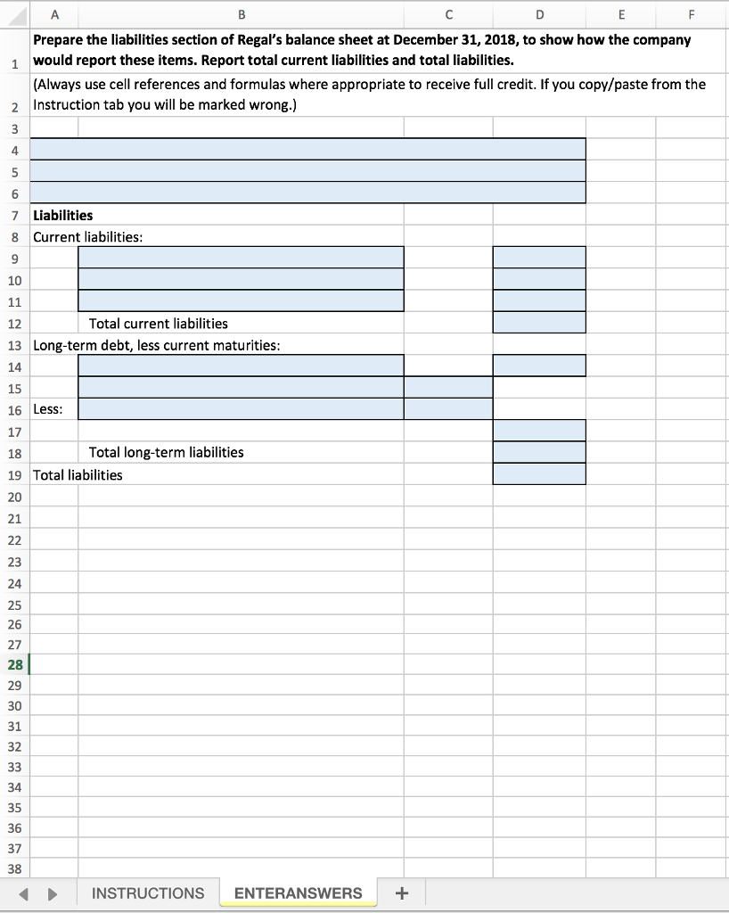


A B Long-term Liabilities Issue bonds payable at a discount and amortize bonds using the effective-interest method 1 2 On March 31, 2019, Pearce Corporation issued bonds payable with characteristics given below. The bonds pay interest semiannually Pearce Corporation's year-end is March 31 4 $ Bonds payable issued Maturity (years) Stated interest rate Market interest rate 580,000 10 6% 10% Use the blue shaded areas on the ENTERANSWERS tab for inputs. Always use cell references and formulas where appropriate to receive full credit. If you copy/paste from the Instruction tab you 11 12 wll be marked wrong 13 15 Requirements 16 1 Using the PV function in Excel, calculate the issue price of the bonds. a. Note that the PMT and FV agruments of the PV function are expected as negative values. Use a value of 0 for the Type argument of the PV function. Enter all amounts as positive values. Do not use a minus sign or parentheses for any values to be subtracted. Use cell references from prior calculations, if applicable. 17 18 2 Prepare an effective-interest amortization table for the bonds through the first three interest payments. a. 19 b. 3 Journalize Pearce Corporation's issuance of the bonds on March 31, 2019, and payment of the first semiannual interest amount and amortization of the bond discount on September 30, 2019 a. Explanations are not required b. Check your spelling carefully and do not abbreviate C. Record debits first, then credits. Exclude explanations from journal entries. d. Use cell references from prior calculations, if applicable. 21 23 25 26 27 28 Saving & Submitting Solution 29 1 Save file to desktop Create folder on desktop, and label COMPLETED EXCEL PROJECTS Save your solution in the folder you just created; add-solution-date to end of file name a. 31 b. 32 2 Upload and submit your file to be graded. a. Navigate back to the activity window screen where you downloaded the initial spreadsheet b. Click Choose button under step 3; locate the file you just saved and click Open c. Click Upload button under step 3 d. Click Submit button under step 4 35 36 37 39 Viewing Results 40 1Click on Results tab in MyAccountingLab 41 2 Click on the Assignment you were working on 42 3 Click on Project link; this will bring up your Score Card 43 4 Within Score Card window, click on Live Comments Report (lower right) to download spreadsheet with feedback 45 46 47 INSTRUCTIONS ENTERANSWERS + 1. Using the PV function in Excel, calculate the issue price of the bonds (Always use cell references and formulas where appropriate to receive full credit. If you copy/paste from the Instruction tab you will be marked wrong.) 1 2 4 Issue price 5 2. Prepare an effective-interest amortization table for the bonds through the first three interest payments. 6 (Always use cell references and formulas where appropriate to receive full credit. If you copy/paste from the Instruction tab you will be marked wrong.) 7 Semiannual Bond Carrying Amount Interest Payment Interest Expense Discount Discount Account Amortization Balance 10 Interest Date 11 Mar. 31, 2019 12 Sep. 30, 2019 13 Mar. 31, 2020 14 Sep. 30, 2020 15 3. Journalize Pearce Corporation's issuance of the bonds on March 31,2019, and payment of the first semiannual 16 interest amount and amortization of the bond discount on September 30, 2019. (Always use cell references and formulas where appropriate to receive full credit. If you copy/paste from the 17 Instruction tab you will be marked wrong.) 18 19 20 Mar. 31, 20159 21 Date Accounts Debit Credit 23 24Sep. 30, 2019 25 26 27 28 1 2 A B Long-Term Liabilities Calculate the leverage ratio, debt ratio, and times-interest-earned ratio, and evaluate debt-paying ability Examine the following selected financial information for The Deal Corporation and Simple Stores, Inc., as of the end of their 4 fiscal years ending in 2018 The Deal Corporation Simple Stores, Inc. In millions 1. Total assets 2. Total common stockholders' equity 3. Operating income 4. Interest expense 5. Leverage ratio 6. Total debt 7. Debt ratio 8. Times interest earned 16,870 $ 203,130 71,310 26,930 2,050 3,080 1,400 $ 87 $ 9 10 12 13 14 15 16 Use the blue shaded areas on the ENTERANSWERS tab for inputs Always use cell references and formulas where appropriate to receive full credit. If you copy/paste from the Instruction tab 17 you will be marked wrong. 18 19 Requirement 20 Complete the table, calculating all the requested information for the two companies 21 Use year-end figures in place of averages where needed for the purpose of calculating the ratios Calculate the debt ratio as a decimal a. b. 23 24 25 Saving & Submitting Solution 26 1 Save file to desktop 27 28 29 2 Upload and submit your file to be graded 30 31 32 a. Create folder on desktop, and label COMPLETED EXCEL PROJECTS b.Save your solution in the folder you just created; add -solution-date to end of file name a.Navigate back to the activity window-screen where you downloaded the initial spreadsheet b. Click Choose button under step 3; locate the file you just saved and click Open c. Click Upload button under step 3 d Click Submit button under step 4 34 35 36 Viewing Results 37 1 Click on Results tab in MyAccountingla!b 38 2 Click on the Assignment you were working on 39 3 Click on Project link; this will bring up your Score Card 4 Within Score Card window, click on Live Comments Report (lower right) to download spreadsheet with feedback 40 Complete the table, calculating all the requested information for the two companies. (Always use cell references and formulas where appropriate to receive full credit. If you copy/paste from the Instruction tab you will be marked wrong.) 1 2 The Deal Corporation Simple Stores, Inc 5 5. Leverage ratio 6 6. Total debt 7 7. Debt ratio 8 8. Times interest earned 10 12 13 14 15 16 17 18 19 20 21 23 24 25 26 27 28 29 30 31 32 34 35 36 37 38 39 40 41 43 INSTRUCTIONS ENTERANSWERS+ A B 1 Long-term Liabilities 2 Report liabilities 4 Regal, Inc., includes the following selected accounts in its general ledger at December 31, 2018 Bonds payable (excluding current portion) Equipment Current portion of bonds payable Notes payable, long-term Interest payable (due March 1, 2019) Accounts payable Discount on bonds payable (all long-term) Accounts receivable $ 400,000 113,000 51,000 275,000 2,000 37,000 12,000 32,000 10 12 13 15 Use the blue shaded areas on the ENTERANSWERS tab for inputs. Always use cell references and formulas where appropriate to receive full credit. If you copy/paste from the Instruction tab you will be 16 marked wrong. 17 18 Requirement Prepare the liabilities section of Regal's balance sheet at December 31,2018, to show how the company would report these items. Report total 19 current liabilities and total liabilities. 20 21 Check your spelling carefully and do not abbreviate. Enter all amounts as positive values. Do not use a minus sign or parentheses for any values to be subtracted. a. b. 23 24 Saving & Submitting Solution 25 1 Save file to desktop 26 27 28 2 Upload and submit your file to be graded. a. Create folder on desktop, and label COMPLETED EXCEL PROJECTS b. Save your solution in the folder you just created; add -solution-date to end of file name a.Navigate back to the activity window screen where you downloaded the initial spreadsheet b. Click Choose button under step 3; locate the file you just saved and click Open c. Click Upload button under step3 d. Click Submit button under step 4 31 32 35 Viewing Results 36 1 Click on Results tab in MyAccountingLab 37 2 Click on the Assignment you were working on 38 3 Click on Project link; this will bring up your Score Card 39 4 Within Score Card window, click on Live Comments Report (lower right) to download spreadsheet with feedback 41 42 43 45 46 47 INSTRUCTIONS ENTERANSWERS + Prepare the liabilities section of Regal's balance sheet at December 31, 2018, to show how the company would report these items. Report total current liabilities and total liabilities. (Always use cell references and formulas where appropriate to receive full credit. If you copy/paste from the 1 2Instruction tab you will be marked wrong.) 7 Liabilities 8 Current liabilities: 10 Total current liabilities 12 13 Long-term debt, less current maturities: 14 15 16 Less: 17 18 19 Total liabilities 20 21 Total long-term liabilities 23 24 25 26 27 28 29 30 31 32 34 35 36 37 38 INSTRUCTIONS ENTERANSWERS+
