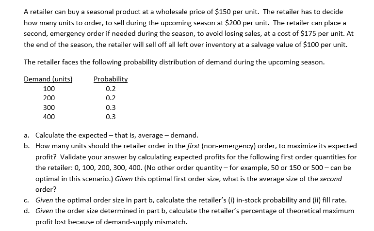
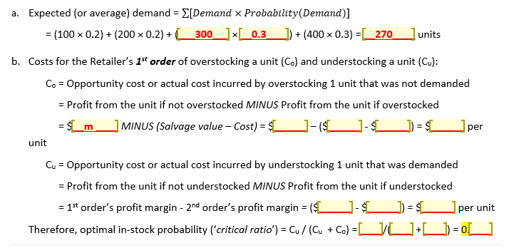
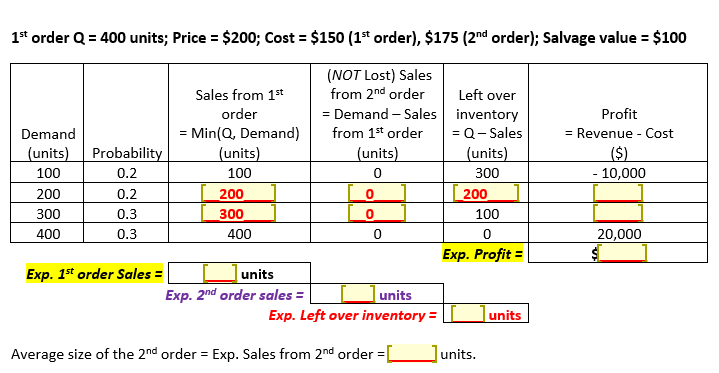
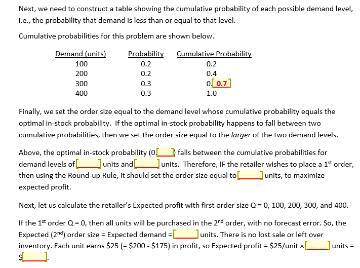
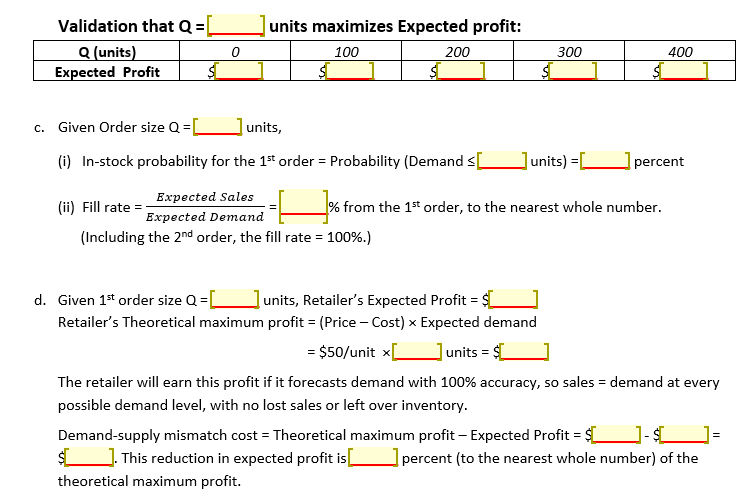
A retailer can buy a seasonal product at a wholesale price of $150 per unit. The retailer has to decide how many units to order, to sell during the upcoming season at $200 per unit. The retailer can place a second, emergency order if needed during the season, to avoid losing sales, at a cost of $175 per unit. At the end of the season, the retailer will sell off all left over inventory at a salvage value of $100 per unit. The retailer faces the following probability distribution of demand during the upcoming season. Demand (units) 100 200 300 400 Probability 0.2 0.2 0.3 0.3 a. Calculate the expected - that is, average - demand. b. How many units should the retailer order in the first (non-emergency) order, to maximize its expected profit? Validate your answer by calculating expected profits for the following first order quantities for the retailer: 0, 100, 200, 300, 400. (No other order quantity for example, 50 or 150 or 500 - can be optimal in this scenario.) Given this optimal first order size, what is the average size of the second order? C. Given the optimal order size in part b, calculate the retailer's (i) in-stock probability and (ii) fill rate. d. Given the order size determined in part b, calculate the retailer's percentage of theoretical maximum profit lost because of demand-supply mismatch. a. Expected (or average) demand = {[Demand x Probability(Demand)] = (100 x 0.2) + (200 x0.2) +_300_]*__0.3_])+(400 x 0.3) =[_270_ units b. Costs for the Retailer's 1st order of overstocking a unit (Co) and understocking a unit (Cu): Co = Opportunity cost or actual cost incurred by overstocking 1 unit that was not demanded = Profit from the unit if not overstocked MINUS Profit from the unit if overstocked = $(_m_] MINUS (Salvage value - Cost) = $C ]-($ per unit Cu = Opportunity cost or actual cost incurred by understocking 1 unit that was demanded = Profit from the unit if not understocked MINUS Profit from the unit if understocked = 1st order's profit margin - 2nd order's profit margin = ($)-$ Therefore, optimal in-stock probability ('critical ratio') = Cu/(Cu + Co) = UU+])=0_ per unit 1st order Q = 400 units; Price = $200; Cost = $150 (1st order), $175 (2nd order); Salvage value = $100 Profit Revenue - Cost ($) - 10,000 (NOT Lost) Sales Sales from 1st from 2nd order Left over order = Demand - Sales inventory Demand = Min(Q, Demand) from 1st order = Q-Sales (units) Probability (units) (units) (units) 100 0.2 100 0 300 200 0.2 200 0 200 300 0.3 300 0 100 400 0.3 400 0 0 Exp. Profit = Exp. 1st order Sales = units Exp. 2nd order sales = units Exp. Left over inventory = units 20,000 Average size of the 2nd order = Exp. Sales from 2nd order = units. Next, we need to construct a table showing the cumulative probability of each possible demand level, i.e., the probability that demand is less than or equal to that level. Cumulative probabilities for this problem are shown below. Demand (units) 100 200 300 Probability 0.2 0.2 0.3 0.3 Cumulative Probability 0.2 0.4 o[_0.7] 1.0 400 Finally, we set the order size equal to the demand level whose cumulative probability equals the optimal in-stock probability. If the optimal in-stock probability happens to fall between two cumulative probabilities, then we set the order size equal to the larger of the two demand levels. Above, the optimal in-stock probability (0) falls between the cumulative probabilities for demand levels of units and units. Therefore, IF the retailer wishes to place a 1st order, then using the Round-up Rule, it should set the order size equal to _units, to maximize expected profit. Next, let us calculate the retailer's Expected profit with first order size Q = 0, 100, 200, 300, and 400. If the 1st order Q = 0, then all units will be purchased in the 2nd order, with no forecast error. So, the Expected (2nd) order size = Expected demand = [units. There is no lost sale or left over inventory. Each unit earns $25 (= $200 - $175) in profit, so Expected profit = $25/unit x $C units = Validation that Q = Q(units) 0 Expected Profit $C units maximizes Expected profit: 100 200 $ SC 300 $1 400 $ C. Given Order size Q=_ 1 units, (i) In-stock probability for the 1st order = Probability (Demands units) = _] percent Expected Sales (ii) Fill rate Expected Demand % from the 1st order, to the nearest whole number. (Including the 2nd order, the fill rate = 100%.) -- d. Given 1st order size Q=L l units, Retailer's Expected Profit = $C Retailer's Theoretical maximum profit = (Price - Cost) Expected demand = $50/unit [units = $_ The retailer will earn this profit if it forecasts demand with 100% accuracy, so sales = demand at every possible demand level, with no lost sales or left over inventory. Demand-supply mismatch cost = Theoretical maximum profit - Expected Profit = $C ]. This reduction in expected profit is percent (to the nearest whole number) of the theoretical maximum profit. A retailer can buy a seasonal product at a wholesale price of $150 per unit. The retailer has to decide how many units to order, to sell during the upcoming season at $200 per unit. The retailer can place a second, emergency order if needed during the season, to avoid losing sales, at a cost of $175 per unit. At the end of the season, the retailer will sell off all left over inventory at a salvage value of $100 per unit. The retailer faces the following probability distribution of demand during the upcoming season. Demand (units) 100 200 300 400 Probability 0.2 0.2 0.3 0.3 a. Calculate the expected - that is, average - demand. b. How many units should the retailer order in the first (non-emergency) order, to maximize its expected profit? Validate your answer by calculating expected profits for the following first order quantities for the retailer: 0, 100, 200, 300, 400. (No other order quantity for example, 50 or 150 or 500 - can be optimal in this scenario.) Given this optimal first order size, what is the average size of the second order? C. Given the optimal order size in part b, calculate the retailer's (i) in-stock probability and (ii) fill rate. d. Given the order size determined in part b, calculate the retailer's percentage of theoretical maximum profit lost because of demand-supply mismatch. a. Expected (or average) demand = {[Demand x Probability(Demand)] = (100 x 0.2) + (200 x0.2) +_300_]*__0.3_])+(400 x 0.3) =[_270_ units b. Costs for the Retailer's 1st order of overstocking a unit (Co) and understocking a unit (Cu): Co = Opportunity cost or actual cost incurred by overstocking 1 unit that was not demanded = Profit from the unit if not overstocked MINUS Profit from the unit if overstocked = $(_m_] MINUS (Salvage value - Cost) = $C ]-($ per unit Cu = Opportunity cost or actual cost incurred by understocking 1 unit that was demanded = Profit from the unit if not understocked MINUS Profit from the unit if understocked = 1st order's profit margin - 2nd order's profit margin = ($)-$ Therefore, optimal in-stock probability ('critical ratio') = Cu/(Cu + Co) = UU+])=0_ per unit 1st order Q = 400 units; Price = $200; Cost = $150 (1st order), $175 (2nd order); Salvage value = $100 Profit Revenue - Cost ($) - 10,000 (NOT Lost) Sales Sales from 1st from 2nd order Left over order = Demand - Sales inventory Demand = Min(Q, Demand) from 1st order = Q-Sales (units) Probability (units) (units) (units) 100 0.2 100 0 300 200 0.2 200 0 200 300 0.3 300 0 100 400 0.3 400 0 0 Exp. Profit = Exp. 1st order Sales = units Exp. 2nd order sales = units Exp. Left over inventory = units 20,000 Average size of the 2nd order = Exp. Sales from 2nd order = units. Next, we need to construct a table showing the cumulative probability of each possible demand level, i.e., the probability that demand is less than or equal to that level. Cumulative probabilities for this problem are shown below. Demand (units) 100 200 300 Probability 0.2 0.2 0.3 0.3 Cumulative Probability 0.2 0.4 o[_0.7] 1.0 400 Finally, we set the order size equal to the demand level whose cumulative probability equals the optimal in-stock probability. If the optimal in-stock probability happens to fall between two cumulative probabilities, then we set the order size equal to the larger of the two demand levels. Above, the optimal in-stock probability (0) falls between the cumulative probabilities for demand levels of units and units. Therefore, IF the retailer wishes to place a 1st order, then using the Round-up Rule, it should set the order size equal to _units, to maximize expected profit. Next, let us calculate the retailer's Expected profit with first order size Q = 0, 100, 200, 300, and 400. If the 1st order Q = 0, then all units will be purchased in the 2nd order, with no forecast error. So, the Expected (2nd) order size = Expected demand = [units. There is no lost sale or left over inventory. Each unit earns $25 (= $200 - $175) in profit, so Expected profit = $25/unit x $C units = Validation that Q = Q(units) 0 Expected Profit $C units maximizes Expected profit: 100 200 $ SC 300 $1 400 $ C. Given Order size Q=_ 1 units, (i) In-stock probability for the 1st order = Probability (Demands units) = _] percent Expected Sales (ii) Fill rate Expected Demand % from the 1st order, to the nearest whole number. (Including the 2nd order, the fill rate = 100%.) -- d. Given 1st order size Q=L l units, Retailer's Expected Profit = $C Retailer's Theoretical maximum profit = (Price - Cost) Expected demand = $50/unit [units = $_ The retailer will earn this profit if it forecasts demand with 100% accuracy, so sales = demand at every possible demand level, with no lost sales or left over inventory. Demand-supply mismatch cost = Theoretical maximum profit - Expected Profit = $C ]. This reduction in expected profit is percent (to the nearest whole number) of the theoretical maximum profit