Accounting Excel Assignment

Instructions are the first 2 pictures, assignment is the last 2 pictures

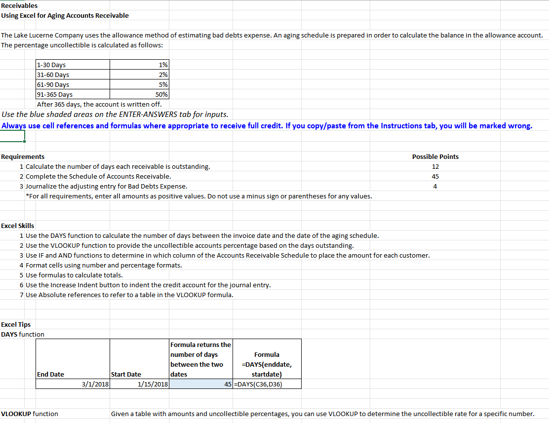
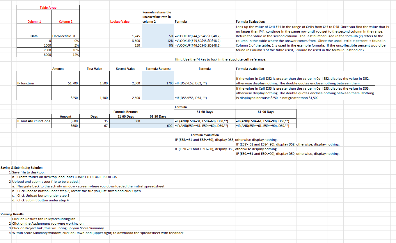
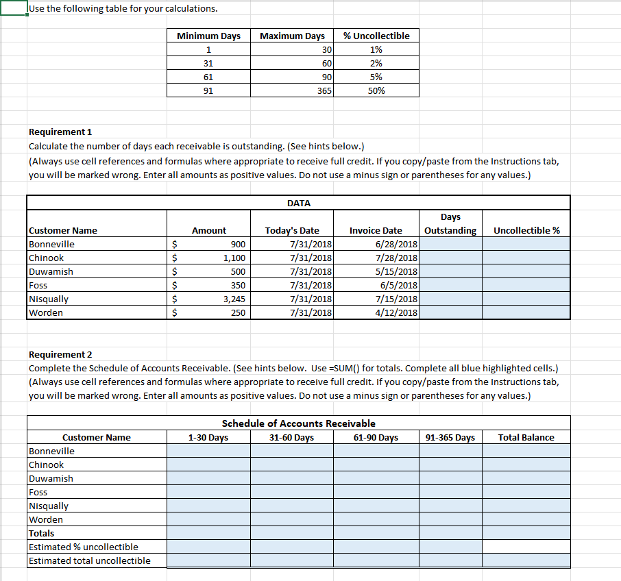
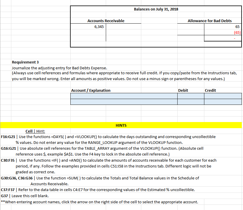
This is all the information I have, any and all help is appreciated

Receivables Using Excel for Aging Accounts Receivable The Lake Lucerne Company uses the allowance method of estimating bad debts expense. An aging schedule is prepared in order to calculate the balance in the allowance account. The percentage uncollectible is calculated as follows: \begin{tabular}{|l|r|} \hline 130 Days & 1% \\ \hline 3160 Days & 2% \\ \hline 6190 Days & 5% \\ \hline 91365 Days & 50% \\ \hline \end{tabular} After 365 days, the account is written off. Use the blue shaded areas on the ENTER-ANSWERS tab for inputs. Always use cell references and formulas where appropriate to receive full credit. If you copy/paste from the Instructions tab, you will be marked wrong. Requirements Possible Points 1 Calculate the number of days each receivable is outstanding. 2 Complete the Schedule of Accounts Receivable. 3 Journalize the adjusting entry for Bad Debts Expense. *For all requirements, enter all amounts as positive values. Do not use a minus sign or parentheses for any values. Excel Skills 1 Use the DAYS function to calculate the number of days between the invoice date and the date of the aging schedule. 2 Use the VLOOKUP function to provide the uncollectible accounts percentage based on the days outstanding. 3 Use IF and AND functions to determine in which column of the Accounts Receivable Schedule to place the amount for each customer. 4 Format cells using number and percentage formats. 5 Use formulas to calculate totals. 6 Use the Increase Indent button to indent the credit account for the journal entry. 7 Use Absolute references to refer to a table in the VLOOKUP formula. Excel Tips DAYS function VLOOKUP function Given a table with amounts and uncollectible percentages, you can use VLOOKUP to determine the uncollectible rate for a specific number. \begin{tabular}{|r|r|} \hline \multicolumn{2}{|c|}{ Table Array } \\ \hline & \\ \hline Column 1 & \multicolumn{2}{|c|}{ Column 2 } \\ \hline Data & \\ \hline 1000 & Uncollectible \% \\ \hline 2000 & 5% \\ \hline 3000 & 10% \\ \hline & 12% \\ \hline \end{tabular} Formula Evaluation: Look up the value of Cell F44 in the range of Cells from C45 to D48. Once you find the value that is no larger than F44, continue in the same row until you get to the second column in the range. Return the value in the second column. The last number used in the formula (2) refers to the column in the table where the answer comes from. Since the uncollectible percent is found in Column 2 of the table, 2 is used in the example formula. If the uncollectible percent would be found in Column 3 of the table used, 3 would be used in the formula instead of 2 . Hint: Use the F4 key to lock in the absolute cell reference. Formula evaluation IF (E58>=31 and E58=61 and E58=31 and E59=61 and E59=31 and E58=61 and E58=31 and E59=61 and E59