ACCT& 202 Lab 2 - Bonds Payable

Objective:

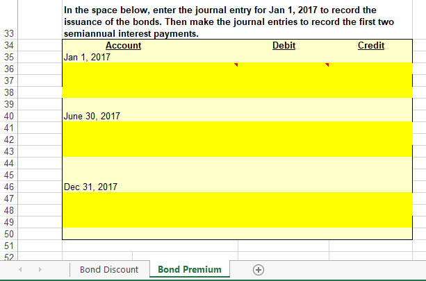
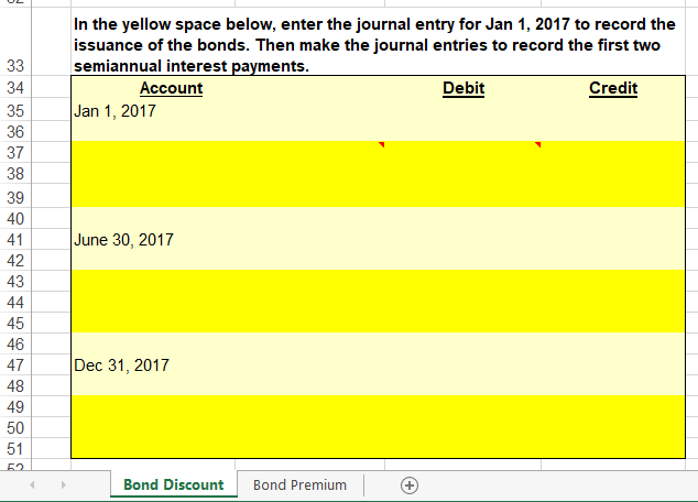
Use Microsoft Excel to calculate the issue price of bonds issued at a discount and bonds issued at a premium, construct an amortization schedule for each of the bond issues, and make the journal entries to record the issuance of the bonds and the first two semiannual interest payments.

Points Possible: 10

Template:

Copy the Excel template for this lab from our course's Canvas website to your desktop or student H: drive. Open the file.

Problem Data:

Bond Discount Problem: On January 1, 2017, Waterfall Lodge & Amusement Park issued $6,000,000 of 6% bonds, due in 10 years. The market interest rate for bonds of similar risk and maturity is 7%. Interest is paid semiannually on June 30 and December 31 each year.

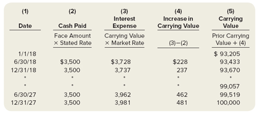
Bond Premium Problem: Assume that the market interest rate is 5.5% instead of 7%. Assume all other given amounts are the same as stated in the bond discount problem.

Required:

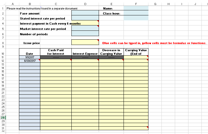
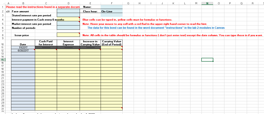
1.Enter the given problem data in the Bond Discount worksheet. Then use the Present Value function in Excel to calculate the issue price of the bonds.

To use the Present Value function, click in cell C7. Type=-PV(

and then use cell references to enter the arguments for the PV function:

The syntax of the PV function is: PV(rate, nper, pmt, [fv], [type])

Rate = Market interest rate, divided by 2 in this problem because interest is paid

semiannually.

Nper = Number of periods.

Pmt = The amount of the semiannual cash interest payment. The formula to calculate is:

Face amount of the bonds x Stated interest rate 2

Fv = Fv stands for future value. When working with bonds, this is the face amount of

the bonds.

Type = Leave this field blank. Doing so indicates payments are made at the end of the

period, which is true for bonds payable.

Check figure: Issue price = $5,573,627.90

Note: Excel will automatically return a negative number. To make it positive you can multiply the formula by negative 1. ( *-1) or put a minus sign in between the = sign and the P( example: =-PV(rate, nper, pmt, [fv], [type])

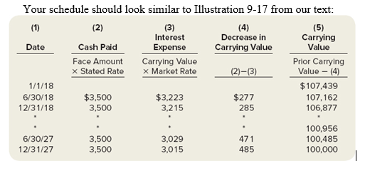
2.Use cell references and Excel formulas to construct an amortization schedule for the entire life of the bonds. Note everything below the data should be a cell reference or formula containing a cell reference. (example"=B4+B5" is ok, =7+4 is not)

Hold your cursor over the red triangles in the corners of selected cells for help creating the formula for that cell.

Your schedule should look similar to Illustration 9-16 from our text: