After reading the instructions, follow steps 1 through 13. When saving the file, add your last name in the filename given in the instructions.
Based on the data in the completed worksheet, design a clustered column chart. Be sure to include chart title, show legends and appropriate axis titles. Move the chart to a new sheet labeled Clustered Chart.
Do Instructions part 3 and complete steps 1 and 2.
When saving the file, add your last name in the filename given in the instructions.
Open a Word document and explain two more Goal Seeking scenarios that can be done using the 8-year financial data.
Save the Word document as Lastname-Mod2.
Submit the two Excel files and the one Word file here.

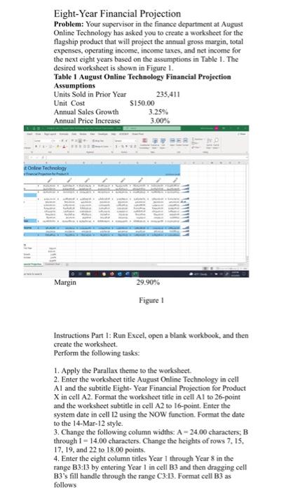
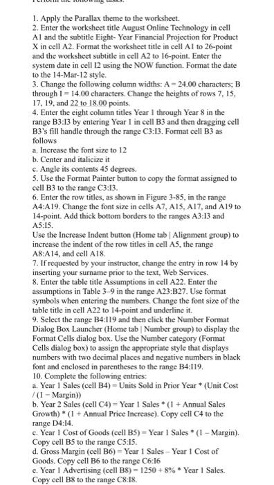
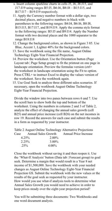
Eight-Year Financial Projection Problem: Your supervisor in the finance department at August Online Technology has asked you to create a worksheet for the flagship product that will project the annual gross margin, total expenses, operating income, income taxes, and net income for the next eight years based on the assumptions in Table 1. The desired worksheet is shown in Figure I. Table 1 August Online Technology Financial Projection Instructions Part 1: Run Excel, open a blank workbook, and then create the worksheet. Perform the following tasks: 1. Apply the Parallax theme to the worksheet. 2. Enter the worksheet title August Online Technology in cell Al and the subtitle Eight- Year Financial Projection for Product X in cell A2. Format the worksheet title in cell A1 to 26-point and the worksheet subtitle in cell A2 to 16-point. Enter the system date in cell 12 using the NOW function. Format the date to the 14-Mar-12 style. 3. Change the following column widths: A24.00 characters; B through I=14.00 characters. Change the heights of rows 7,15 , 17,19 , and 22 to 18,00 points. 4. Enter the cight column titles Year 1 through Year 8 in the range B3:13 by entering Year 1 in cell B3 and then dragging cell B3 's fill handle through the range C3:13. Format cell B3 as follows 1. Apply the Parallax theme to the worksheet. 2. Enter the worksheet title August Online Technology in cell Al and the subtitle Eight- Year Financial Projection for Product X in cell A2. Format the worksheet title in cell Al to 26-point and the worksheet subtitle in cell A2 to 16-point. Enter the system date in cell 12 using the NOW function. Format the date to the 14-Mar-12 style. 3. Change the following column widths: A=24.00 characters; B through I=14.00 characters. Change the heights of rows 7,15 , 17,19 , and 22 to 18.00 points. 4. Enter the eight column titles Year 1 through Year 8 in the range B3:I3 by entering Year 1 in cell B3 and then dragging cell B3 's fill handle through the range C3:13. Format cell B3 as follows a. Increase the font size to 12 b. Center and italicize it c. Angle its contents 45 degrees. 5. Use the Format Painter button to copy the format assigned to cell B3 to the range C3:13. 6. Enter the row titles, as shown in Figure 3-85, in the range A4:A19. Change the font size in cells A7, A15, A17, and A19 to 14-point. Add thick bottom borders to the ranges A3:13 and A5:I5. Use the Increase Indent button (Home tab | Alignment group) to increase the indent of the row titles in cell A5, the range A8:A14, and cell A18. 7. If requested by your instructor, change the entry in row 14 by inserting your surname prior to the text, Web Services. 8. Enter the table title Assumptions in cell A22. Enter the assumptions in Table 3-9 in the range A23:B27. Use format symbols when entering the numbers. Change the font size of the table title in cell A22 to 14-point and underline it. 9. Select the range B4:I19 and then click the Number Format Dialog Box Launcher (Home tab | Number group) to display the Format Cells dialog box. Use the Number category (Format Cells dialog box) to assign the appropriate style that displays numbers with two decimal places and negative numbers in black font and enclosed in parentheses to the range B4:I19. 10. Complete the following entries: a. Year 1 Sales (cell B4) = Units Sold in Prior Year * (Unit Cost /(1 Margin )) b. Year 2 Sales ( cell C4 )= Year 1 Sales * (1+ Annual Sales Growth) * (1+ Annual Price Increase). Copy cell C4 to the range D4:14. c. Year 1 Cost of Goods (cell B5) = Year 1 Sales * (1 Margin ). Copy cell B5 to the range C5:15. d. Gross Margin (cell B6) = Year 1 Sales - Year 1 Cost of Goods. Copy cell B6 to the range C6:16 e. Year 1 Advertising (cell B8) =1250+8% Year I Sales. Copy cell B8 to the range C8:18. 1. Apply the Parallax theme to the worksheet. 2. Enter the worksheet title August Online Technology in cell Al and the subtitle Eight- Year Financial Projection for Product X in cell A2. Format the worksheet title in cell Al to 26-point and the worksheet subtitle in cell A2 to 16-point. Enter the system date in cell 12 using the NOW function. Format the date to the 14-Mar-12 style. 3. Change the following column widths: A=24.00 characters; B through I=14.00 characters. Change the heights of rows 7,15 , 17,19 , and 22 to 18.00 points. 4. Enter the eight column titles Year 1 through Year 8 in the range B3:I3 by entering Year 1 in cell B3 and then dragging cell B3 's fill handle through the range C3:13. Format cell B3 as follows a. Increase the font size to 12 b. Center and italicize it c. Angle its contents 45 degrees. 5. Use the Format Painter button to copy the format assigned to cell B3 to the range C3:13. 6. Enter the row titles, as shown in Figure 3-85, in the range A4:A19. Change the font size in cells A7, A15, A17, and A19 to 14-point. Add thick bottom borders to the ranges A3:13 and A5:I5. Use the Increase Indent button (Home tab | Alignment group) to increase the indent of the row titles in cell A5, the range A8:A14, and cell A18. 7. If requested by your instructor, change the entry in row 14 by inserting your surname prior to the text, Web Services. 8. Enter the table title Assumptions in cell A22. Enter the assumptions in Table 3-9 in the range A23:B27. Use format symbols when entering the numbers. Change the font size of the table title in cell A22 to 14-point and underline it. 9. Select the range B4:I19 and then click the Number Format Dialog Box Launcher (Home tab | Number group) to display the Format Cells dialog box. Use the Number category (Format Cells dialog box) to assign the appropriate style that displays numbers with two decimal places and negative numbers in black font and enclosed in parentheses to the range B4:I19. 10. Complete the following entries: a. Year 1 Sales (cell B4) = Units Sold in Prior Year * (Unit Cost /(1 Margin )) b. Year 2 Sales ( cell C4 )= Year 1 Sales * (1+ Annual Sales Growth) * (1+ Annual Price Increase). Copy cell C4 to the range D4:14. c. Year 1 Cost of Goods (cell B5) = Year 1 Sales * (1 Margin ). Copy cell B5 to the range C5:15. d. Gross Margin (cell B6) = Year 1 Sales - Year 1 Cost of Goods. Copy cell B6 to the range C6:16 e. Year 1 Advertising (cell B8) =1250+8% Year I Sales. Copy cell B8 to the range C8:18. s. Insert column sparkline charts in cells J5, J6, J8.J15, and J17:J19 using ranges B5:15,B6:16,B8:18B15:115, and B17:117-B19:119 respectively. 11. Apply the Currency number format with a dollar sign, two decimal places, and negative numbers in black with parentheses to the following ranges: B4:14, B6:16, B8:I8, B15:115, B17:117, and B19:119. Apply the comma style format to the following ranges: B5:15 and B9:114. Apply the Number format with two decimal places and the 1000 separator to the range B18:118 12. Change the background colors, as shown in Figure 385 . Use Blue, Accent 1, Lighter 40% for the background colors. 13. Save the workbook using the file name, August Online Technology Eight-Year Financial Projection. 14. Preview the worksheet. Use the Orientation button (Page Layout tab | Page Setup group) to fit the printout on one page in landscape orientation. Preview the formulas version (etrl+ the worksheet in landscape orientation using the Fit to option. Press CTRL + to instruct Excel to display the values version of the worksheet. Save the workbook again. 15. Use Goal Seek to analyze three different sales scenarios. If necessary, open the workbook August Online Technology Eight-Year Financial Projection. Divide the window into two panes between rows 6 and 7. Use the scroll bars to show both the top and bottom of the worksheet. Using the numbers in columns 2 and 3 of Table 2. analyze the effect of changing the annual sales growth (cell B25) and annual price increase (cell B26) on the net incomes in row 19. Record the answers for each case and submit the results in a form as requested by your instructor. al Price increase Close the workbook without saving it and then reopen it. Use the 'What-If Analysis' button (Data tab | Forecast group) to goal seek. Determine a margin that would result in a Year 8 net income of $1,500,000. Save the workbook with your needed changes as August Online Technology Eight-Year Financial Projection GS. Submit the workbook with the new values or the results of the goal seek as requested by your instructor. How would you use what-if analysis tools to determine what Annual Sales Growth you would need to achieve in order to keep prices steady over the eight-year projection period? You will be submitting three documents: Two Workbooks and one word document analysis


