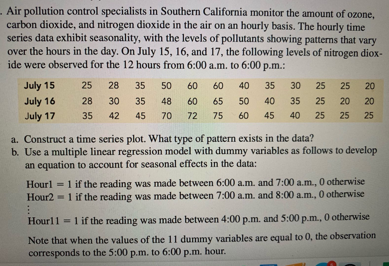
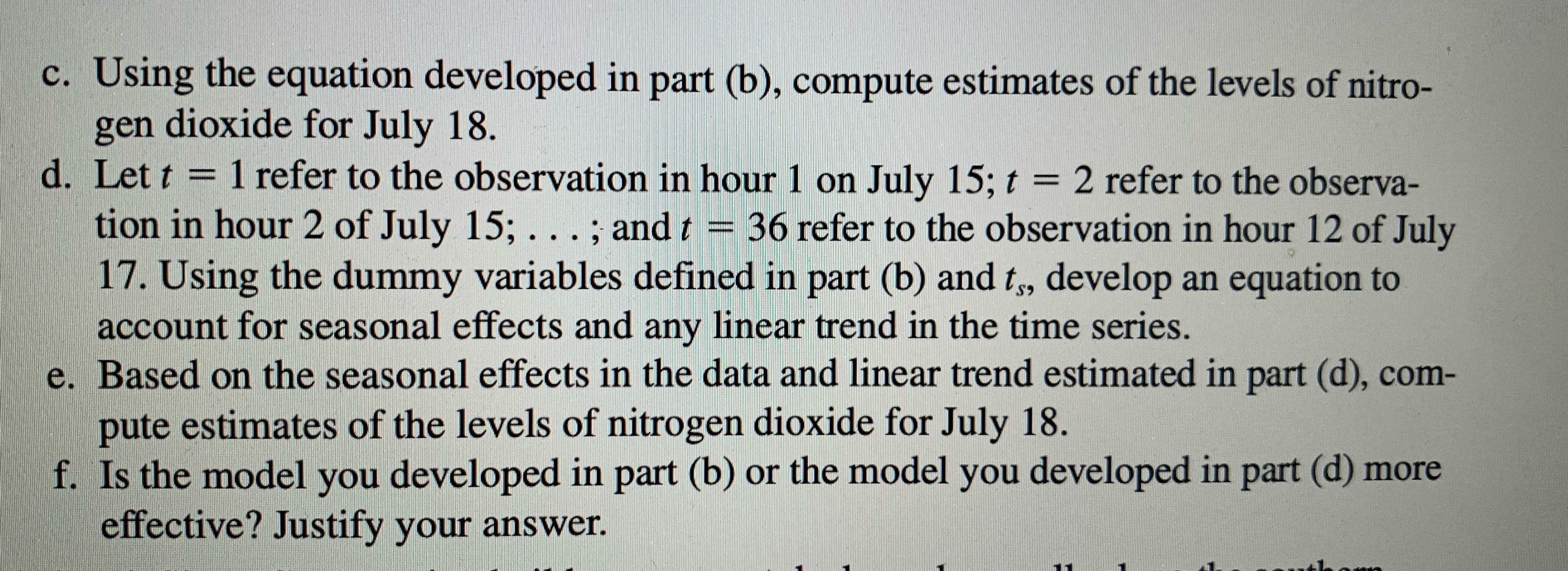
Air pollution control specialists in Southern California monitor the amount of ozone, carbon dioxide, and nitrogen dioxide in the air on an hourly basis. The hourly time series data exhibit seasonality, with the levels of pollutants showing patterns that vary over the hours in the day. On July 15, 16, and 17, the following levels of nitrogen diox- ide were observed for the 12 hours from 6:00 a.m. to 6:00 p.m.: July 15 25 28 35 50 60 60 40 35 30 25 25 20 July 16 28 30 35 48 60 65 50 40 35 25 20 20 July 17 35 42 45 70 72 75 60 45 40 25 25 25 a. Construct a time series plot. What type of pattern exists in the data? b. Use a multiple linear regression model with dummy variables as follows to develop an equation to account for seasonal effects in the data: Hourl = 1 if the reading was made between 6:00 a.m. and 7:00 a.m., 0 otherwise Hour2 = 1 if the reading was made between 7:00 a.m. and 8:00 a.m., 0 otherwise . . Hour1 1 = 1 if the reading was made between 4:00 p.m. and 5:00 p.m., 0 otherwise Note that when the values of the 11 dummy variables are equal to 0, the observation corresponds to the 5:00 p.m. to 6:00 p.m. hour.c. Using the equation developed in part (b), compute estimates of the levels of nitro- gen dioxide for July 18. d. Let t = 1 refer to the observation in hour 1 on July 15; t = 2 refer to the observa- tion in hour 2 of July 15; . . .; and t = 36 refer to the observation in hour 12 of July 17. Using the dummy variables defined in part (b) and t,, develop an equation to account for seasonal effects and any linear trend in the time series. e. Based on the seasonal effects in the data and linear trend estimated in part (d), com- pute estimates of the levels of nitrogen dioxide for July 18. f. Is the model you developed in part (b) or the model you developed in part (d) more effective? Justify your