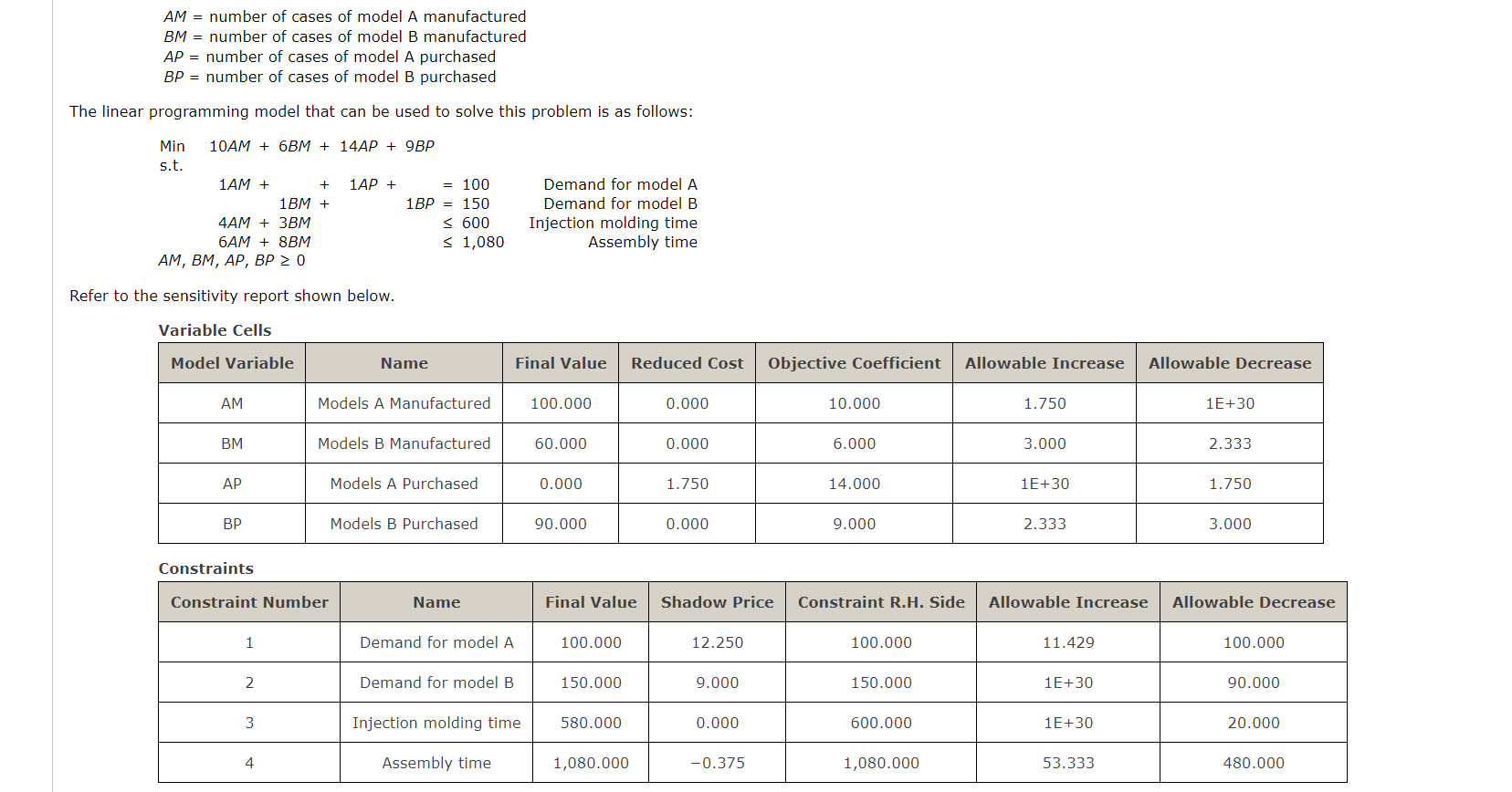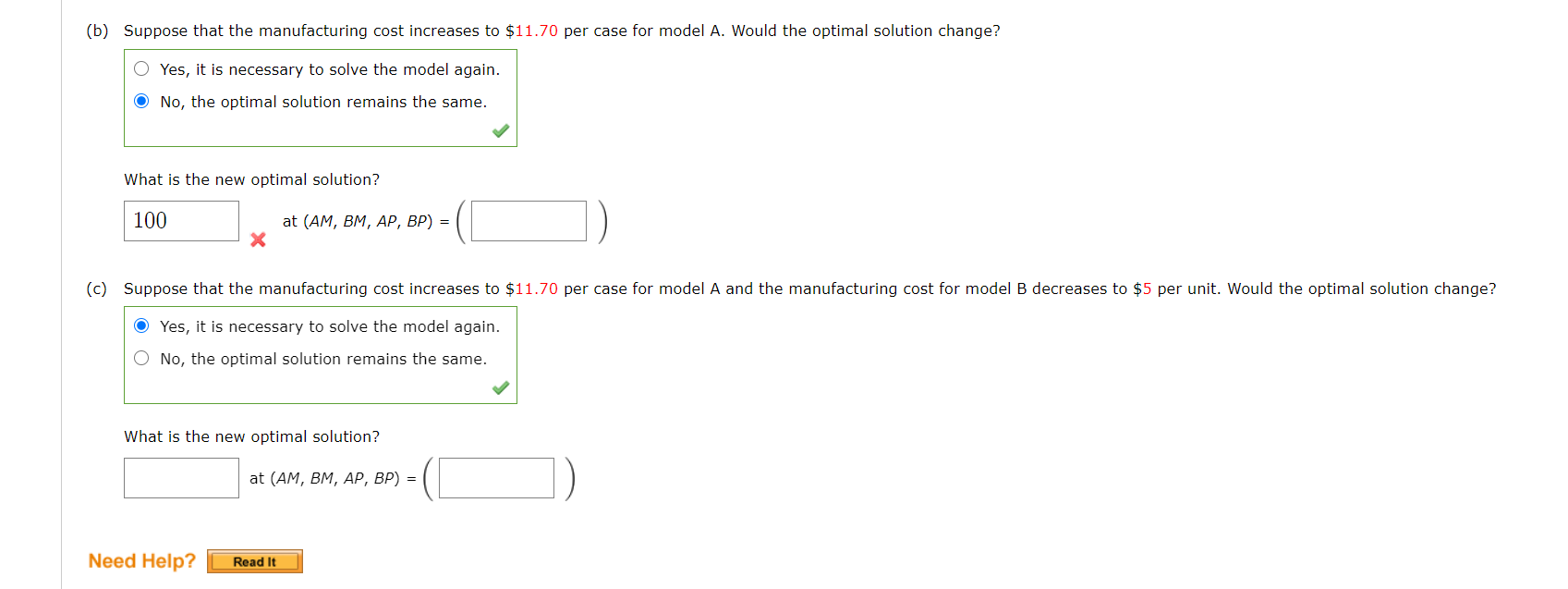

AM = number of cases of model A manufactured BM = number of cases of model B manufactured AP = number of cases of model A purchased BP = number of cases of model B purchased The linear programming model that can be used to solve this problem is as follows: + Min 10AM + 6BM + 14AP + 9BP s.t. 1AM + 1AP + = 100 1BM + 1 BP = 150 4AM + 3BM 0 Demand for model A Demand for model B Injection molding time Assembly time Refer to the sensitivity report shown below. Variable Cells Model Variable Name Final Value Reduced Cost Objective Coefficient Allowable Increase Allowable Decrease AM Models A Manufactured 100.000 0.000 10.000 1.750 1E+30 BM Models B Manufactured 60.000 0.000 6.000 3.000 2.333 Models A Purchased 0.000 1.750 14.000 1E+30 1.750 BP Models B Purchased 90.000 0.000 9.000 2.333 3.000 Constraints Constraint Number Name Final Value Shadow Price Constraint R.H. Side Allowable Increase Allowable Decrease 1 Demand for model A 100.000 12.250 100.000 11.429 100.000 2 Demand for model B 150.000 9.000 150.000 1E+30 90.000 3 Injection molding time 580.000 0.000 600.000 1E+30 20.000 4 Assembly time 1,080.000 -0.375 1,080.000 53.333 480.000 (b) Suppose that the manufacturing cost increases to $11.70 per case for model A. Would the optimal solution change? Yes, it is necessary to solve the model again. No, the optimal solution remains the same. What is the new optimal solution? 100 at (AM, BM, AP, BP) = X (c) Suppose that the manufacturing cost increases to $11.70 per case for model A and the manufacturing cost for model B decreases to $5 per unit. Would the optimal solution change? Yes, it is necessary to solve the model again. O No, the optimal solution remains the same. What is the new optimal solution? at (AM, BM, AP, BP) = Need Help? Read It AM = number of cases of model A manufactured BM = number of cases of model B manufactured AP = number of cases of model A purchased BP = number of cases of model B purchased The linear programming model that can be used to solve this problem is as follows: + Min 10AM + 6BM + 14AP + 9BP s.t. 1AM + 1AP + = 100 1BM + 1 BP = 150 4AM + 3BM 0 Demand for model A Demand for model B Injection molding time Assembly time Refer to the sensitivity report shown below. Variable Cells Model Variable Name Final Value Reduced Cost Objective Coefficient Allowable Increase Allowable Decrease AM Models A Manufactured 100.000 0.000 10.000 1.750 1E+30 BM Models B Manufactured 60.000 0.000 6.000 3.000 2.333 Models A Purchased 0.000 1.750 14.000 1E+30 1.750 BP Models B Purchased 90.000 0.000 9.000 2.333 3.000 Constraints Constraint Number Name Final Value Shadow Price Constraint R.H. Side Allowable Increase Allowable Decrease 1 Demand for model A 100.000 12.250 100.000 11.429 100.000 2 Demand for model B 150.000 9.000 150.000 1E+30 90.000 3 Injection molding time 580.000 0.000 600.000 1E+30 20.000 4 Assembly time 1,080.000 -0.375 1,080.000 53.333 480.000 (b) Suppose that the manufacturing cost increases to $11.70 per case for model A. Would the optimal solution change? Yes, it is necessary to solve the model again. No, the optimal solution remains the same. What is the new optimal solution? 100 at (AM, BM, AP, BP) = X (c) Suppose that the manufacturing cost increases to $11.70 per case for model A and the manufacturing cost for model B decreases to $5 per unit. Would the optimal solution change? Yes, it is necessary to solve the model again. O No, the optimal solution remains the same. What is the new optimal solution? at (AM, BM, AP, BP) = Need Help? Read It
