Answer all questions.,,,

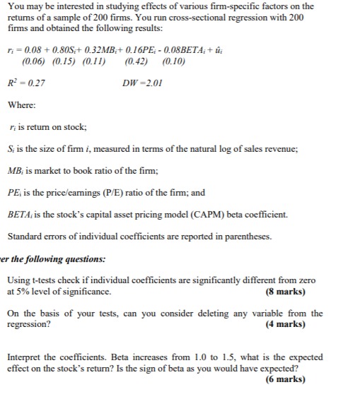
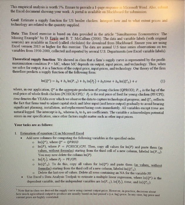
You may be interested in studying effects of various firm-specific factors on the returns of a sample of 200 firms. You run cross-sectional regression with 200 firms and obtained the following results: ri = 0.08 + 0.805,+ 0.32MB;+ 0.16PE: - 0.08BETA; + ui (0.06) (0.15) (0.11) (0.42) (0.10) R- = 0.27 DW =2.01 Where: If is return on stock; S: is the size of firm i, measured in terms of the natural log of sales revenue; MB; is market to book ratio of the firm; PE: is the price/earnings (P/E) ratio of the firm; and BETA, is the stock's capital asset pricing model (CAPM) beta coefficient. Standard errors of individual coefficients are reported in parentheses. er the following questions: Using t-tests check if individual coefficients are significantly different from zero at 5% level of significance. (8 marks) On the basis of your tests, can you consider deleting any variable from the regression? (4 marks) Interpret the coefficients. Beta increases from 1.0 to 1.5, what is the expected effect on the stock's return? Is the sign of beta as you would have expected? (6 marks)This empirical analysis is worth 5%. Ensure to provide a 1-page response in Microsoft Word. Also, submit the Excel document showing your work. A portal is available on Blackboard for submission. Goal: Estimate a supply function for US broiler chicken. Interpret how and to what extent prices and technology are related to the quantity supplied. Data: This Excel exercise is based on data provided in the article "Simultaneous Econometrics: The Missing Example" by D. Epple and B. T. Mccallum (2006). The data and variable labels (with original sources) are available in Excel (called chickdata) for download from Blackboard. Ensure you are using Excel version 2013 or higher for this exercise. The data are annual U.S time series observations on ten variables from 1950-2000, collected and reported by several U.S. Departments (see Excel variable labels). Theoretical supply function: We showed in class that a firm's supply curve is represented by the profit- maximization condition P = MC, where MC depends on output, input prices, and technology. Thus, when we solve for output, it is a function of the output price, input prices, and technology. Our theory of the firm therefore predicts a supply function of the following form: In(Q') = bo + b, In(P_;) + by In(P,) + bytime + b, In(Q=,) + e (1) where, in our application, Q" is the aggregate production of young chicken (QPROD); P_, is the lag of the real price of whole fresh chicken (PCHICK/CPI); P, is the real price of feed for young chicken (PF/CPI); time denotes the YEARs over which we observe the data to capture technological progress; and Q", reflects the fact that firms tend to adjust capital stock and labor input (and hence output) gradually to avoid bearing significant planning, installation, and replacement/hiring costs immediately. All variables except time are natural logged. The intercept is bo. whereas by to be are coefficients. The variable e acknowledges potential errors in our specification, since other factors might matter such as other input prices. Your tasks are as follows: 1. Estimation of equation (1) in Microsoft Excel . Add new columns for computing the following variables in the specified order. o In(Q"), where Q" = QPROD o In(P), where P = PCHICK/CPI. Then, copy all values for In(P) and paste them (as values, without formulas) starting from the third cell of a new column, labeled In(P-,). You may now delete the column In (P). In(P, ). where P, = PF/CPI. In(Q2,). To do this, copy all values for In(Q*) and paste them (as values, without formulas) starting from the third cell of a new column, labeled In(Q#1)- o Delete the last row of values. Delete all rows containing an NA for the variable PF. Use Excel's Data Analysis Toolpak to estimate a multiple linear regression, where In((*) is the dependent variable, and the independent variables are In(P-, ). In(P, ). time, and In(Q- 1) Note that in class we derived the supply curve using current output price. However, in practice, decisions about how much agricultural output to produce are usually based on last period's (ie. lag) price. In any case, lag price and current price are highly correlated.b) Suppose the following relationships are reasonable models of stock market returns in three different markets: Me = 0.7ys1 +0.3ymz + us (5.1) Ve = 0.3Had + ur (5.2) : =0.8 yr1 +0.6 yo2 + 0.3up + 1, (5.3) Answer the following questions: (i) What class of time series models do the equations (5.1). (5.2), and (5.3) belong? (5 marks) (ii) Comment on the expected shapes of the ACF and PACF of each of these processes. (7 marks) c) Outline and discuss in detail the steps suggested by Box and Jenkins (1976) in constructing an ARMA model. (9 marks) d) Explain why it is important to test for non-stationarity in time series data before attempting to build an empirical model. (7 marks)Solve the following queueing theory problems. Submit your complete solutions Zifoshi is a PhD student at University of'uv'isconsin Madison. He does odd jobs to supplement his income. Job requests come every 5 days on the average, but the time between requests is exponential. The time for completing a job is also exponential with mean 4 days. {a} What is the probability that Yoshi will be out of jobs? {b} If Yoshi gets about $50 a job, what is his average monthly income? {c} If at the end of the semester, Yoshi decides to subcontract on the outstanding jobs at $40 each. How much, on the average, should he expect to pay? 36) Determine which one of the following statements regarding guarantees on variable annuity products is FALSE: (A) A guaranteed minimum death benefit (GMDB) with a return of premium guarantee is similar to a European put option with expiration contingent on the death of the policyholder or annuitant. (B) A guaranteed minimum accumulation benefit (GMAB) with a return of premium guarantee is similar to a European put option with payment contingent on the policyholder surviving to the guarantee expiration date and the policy still being in force at that time. (C) A guaranteed minimum withdrawal benefit (GMWB) provides a guarantee that the account value will not be less than the guaranteed withdrawal benefit base at any future time. (D) A guaranteed minimum income benefit (GMIB) provides a guarantee on the future purchase rate for a traditional annuity. (E) An earnings-enhanced death benefit is an optional benefit available with some variable annuity products that acts as a European call option with strike price equal to the original amount invested