Answer the question shown below.

Notes for reference shown below.

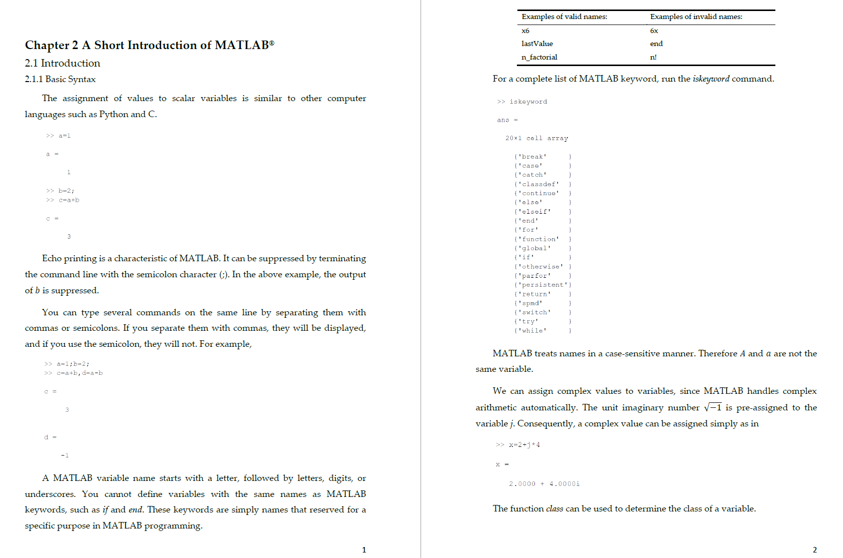
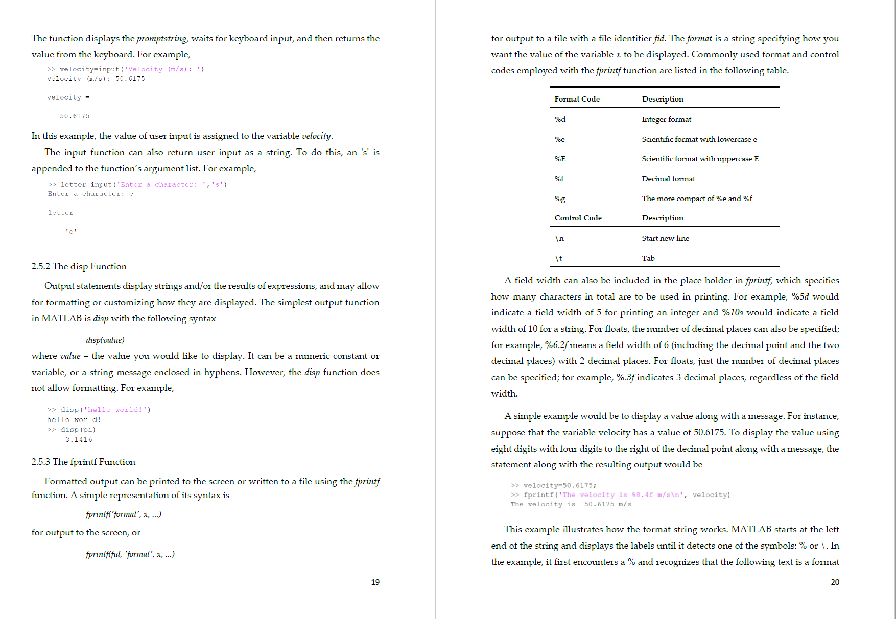
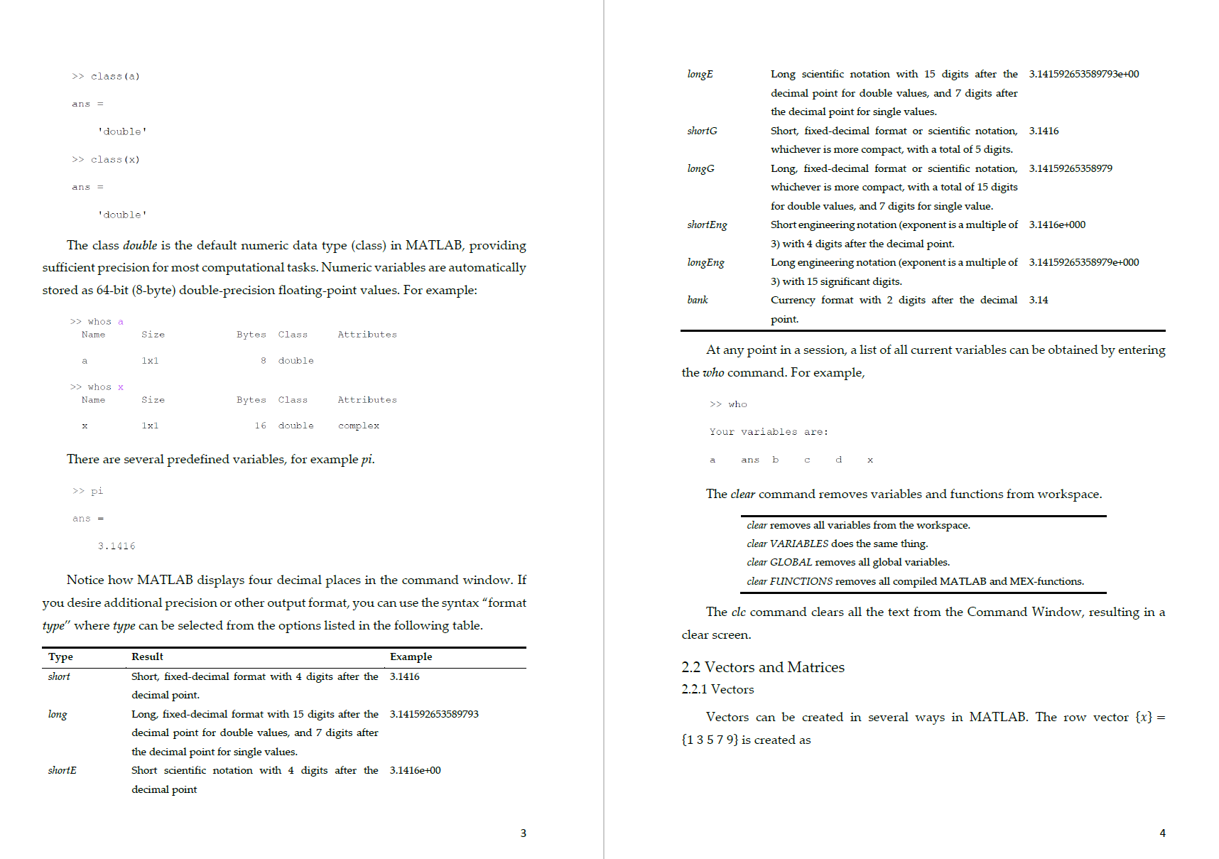
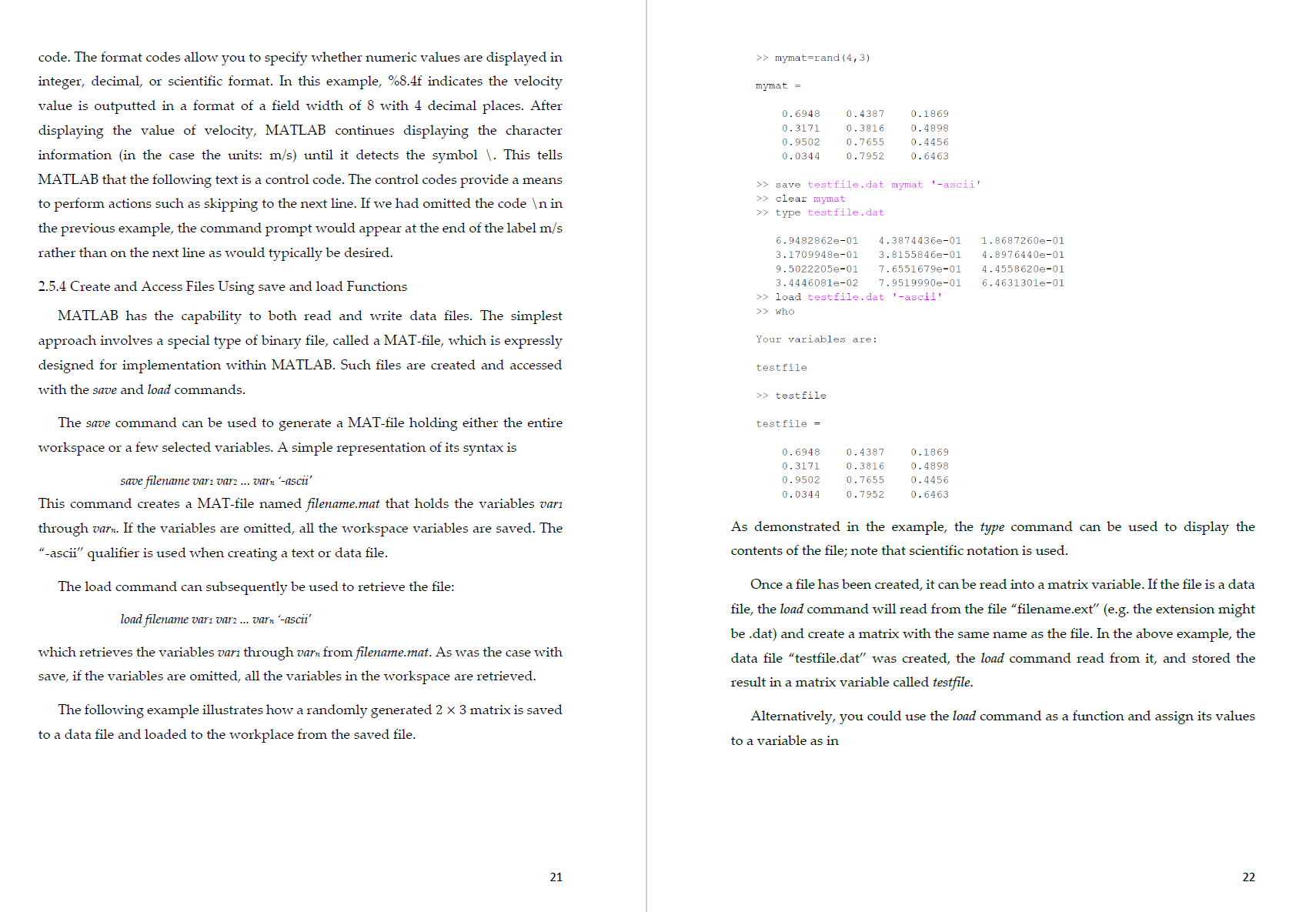
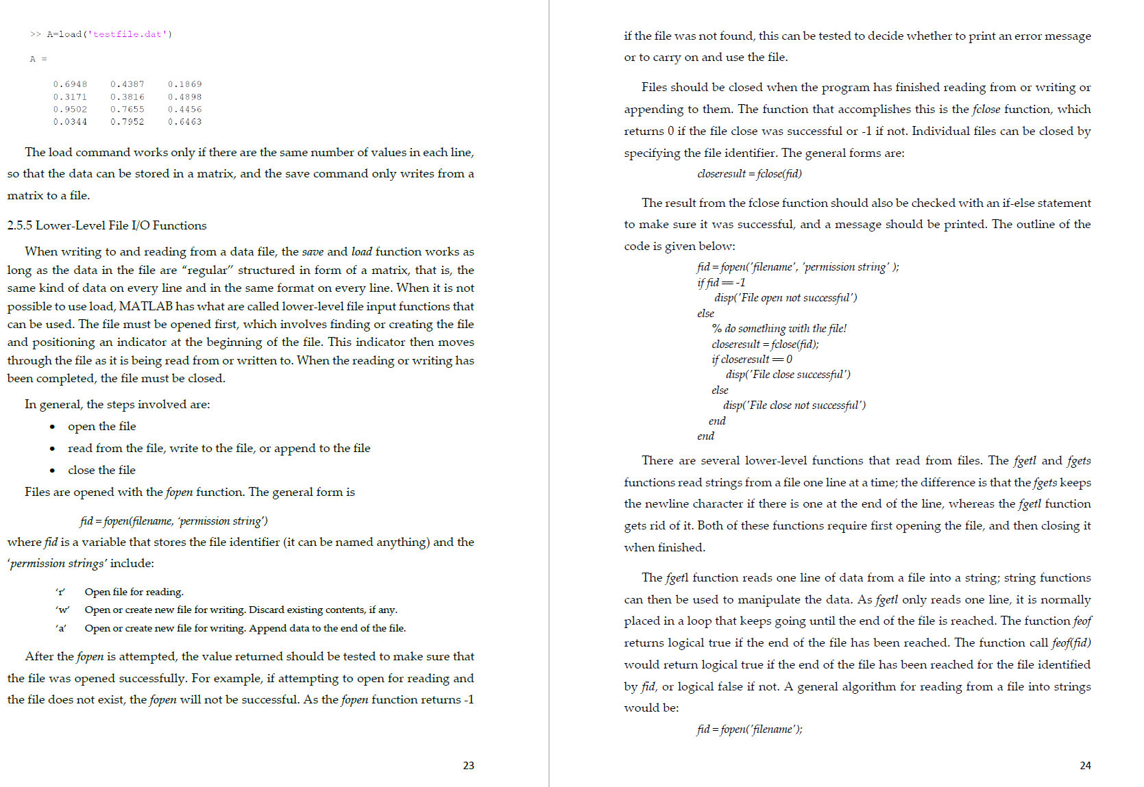
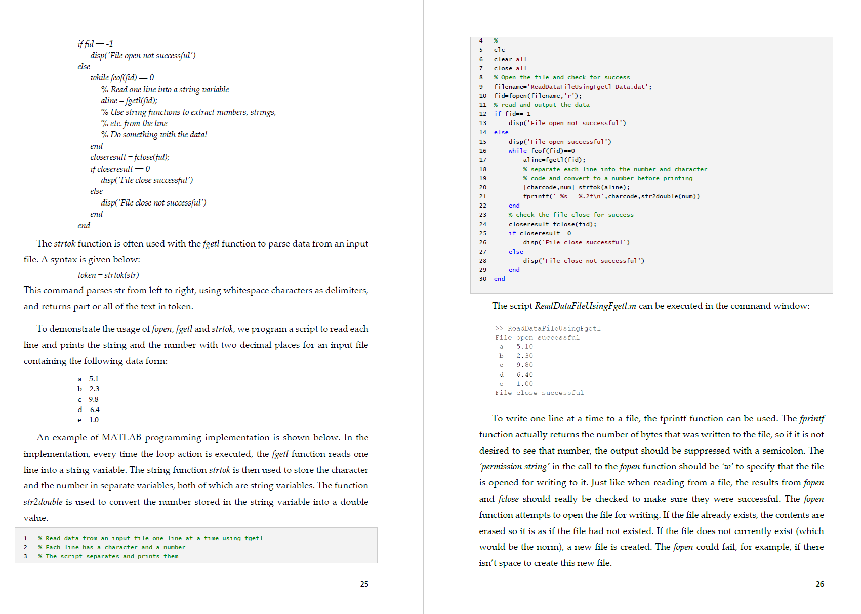
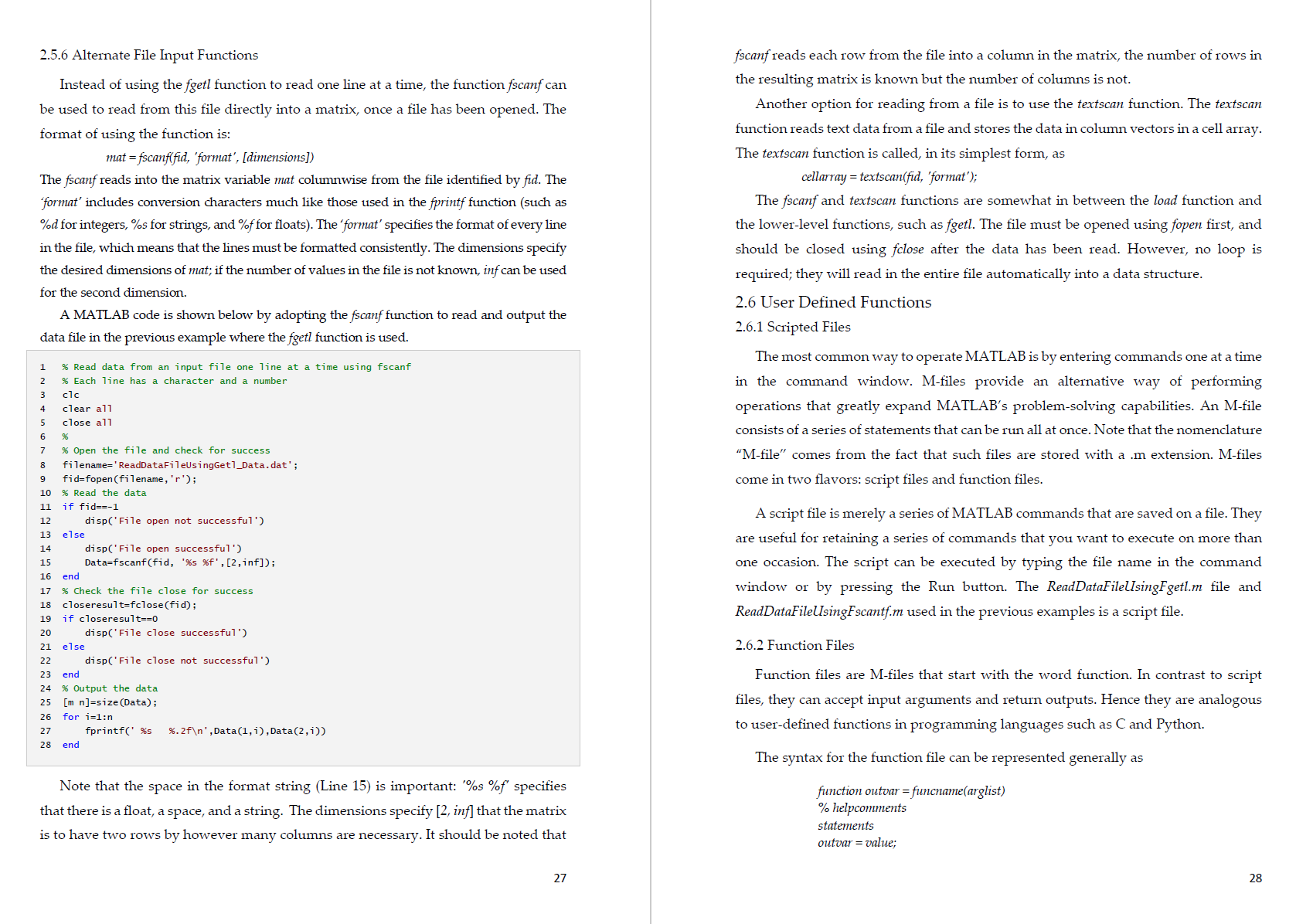
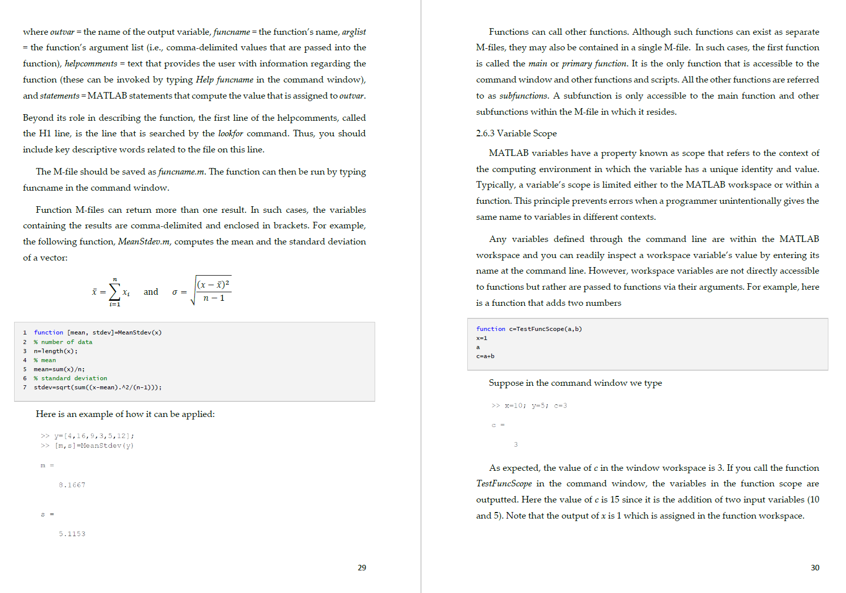
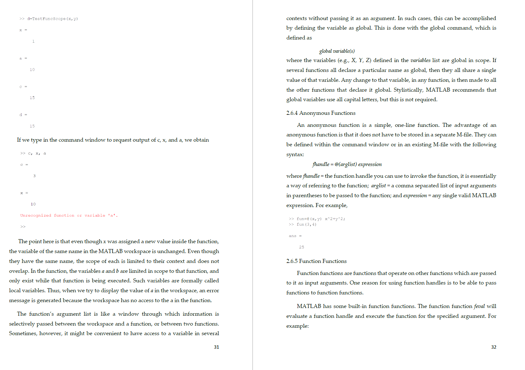
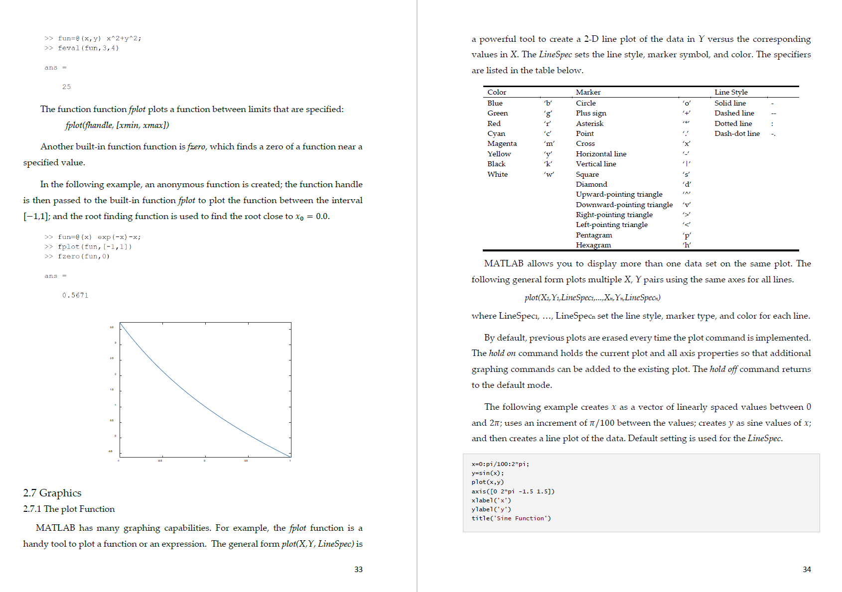
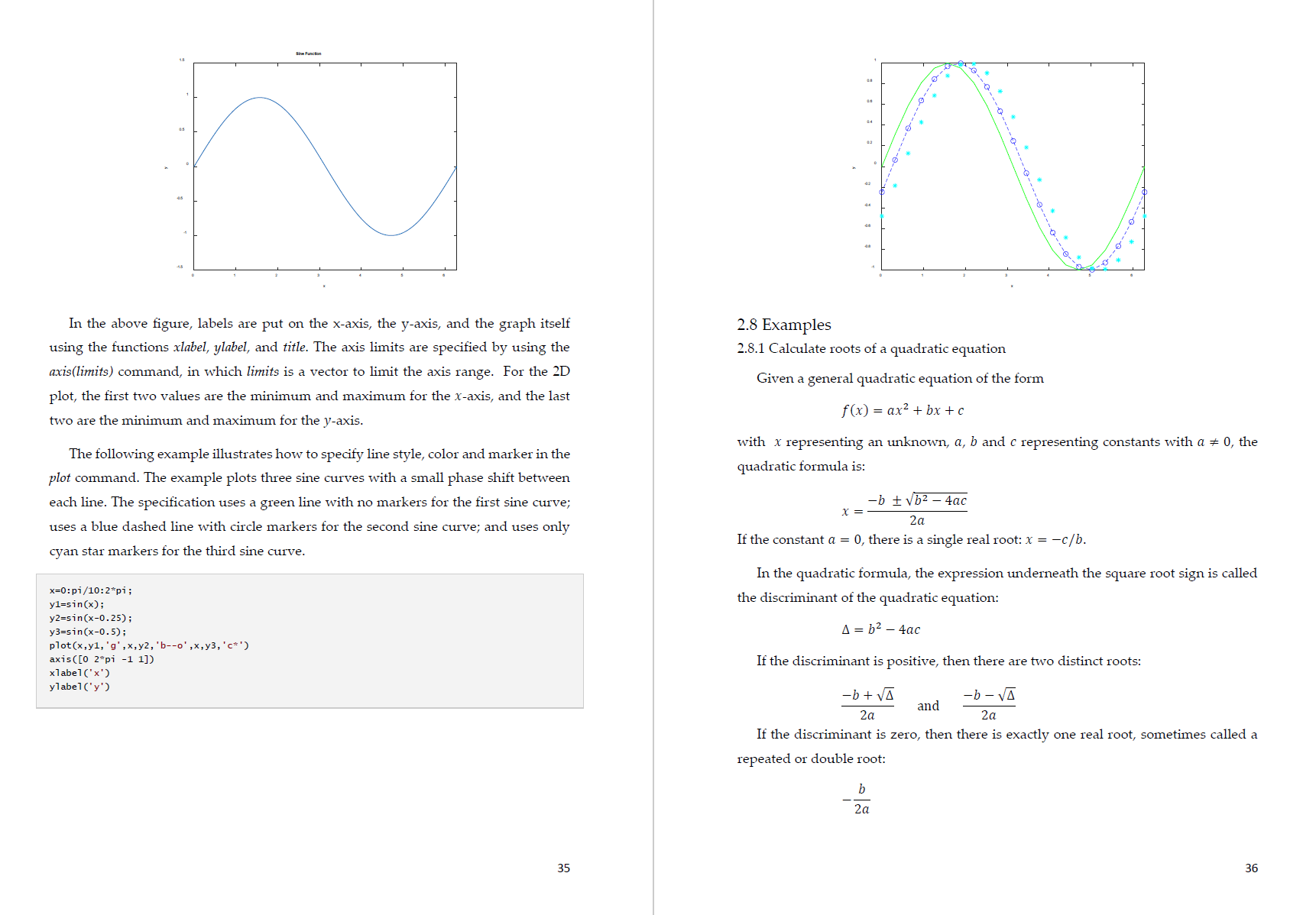
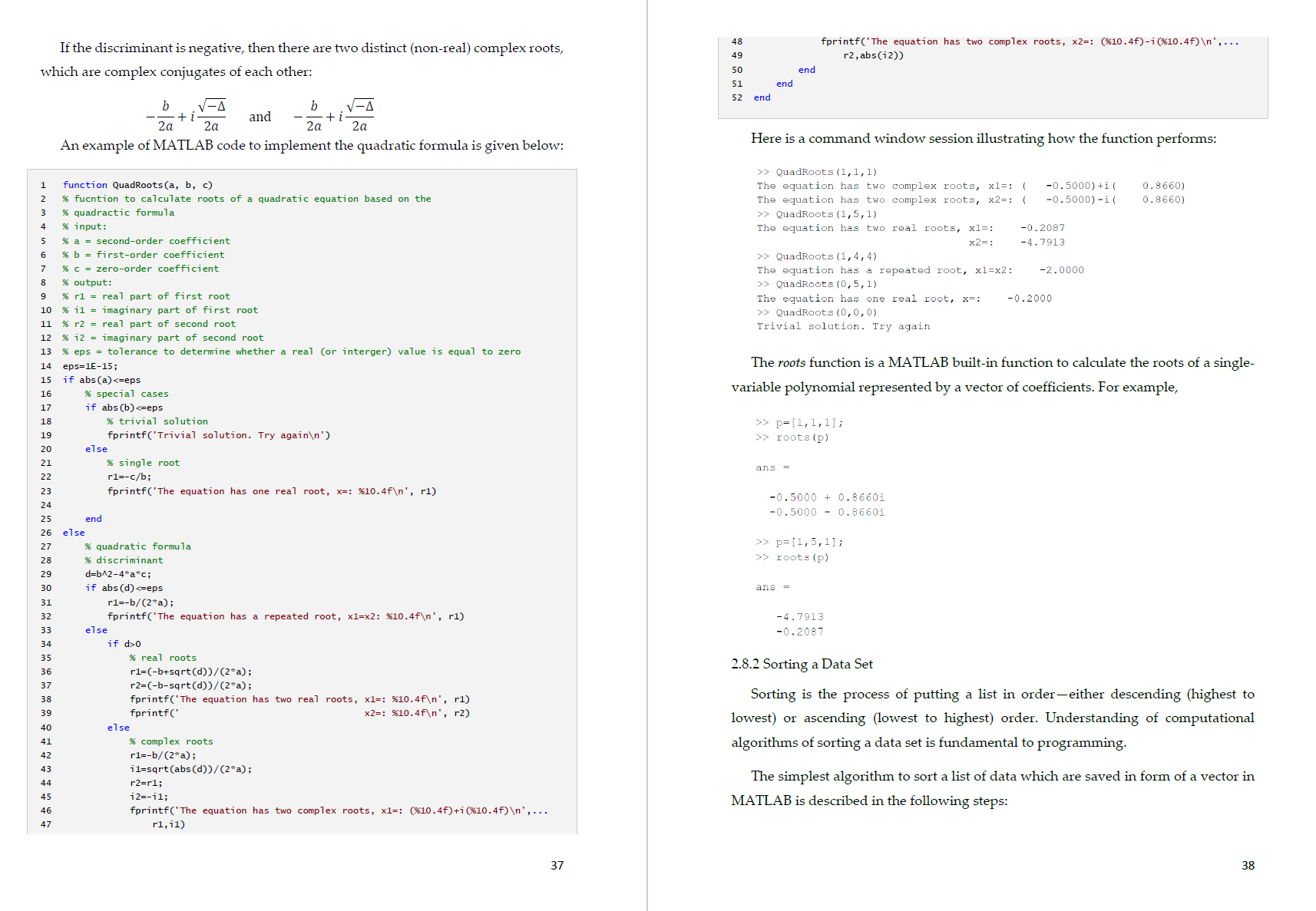
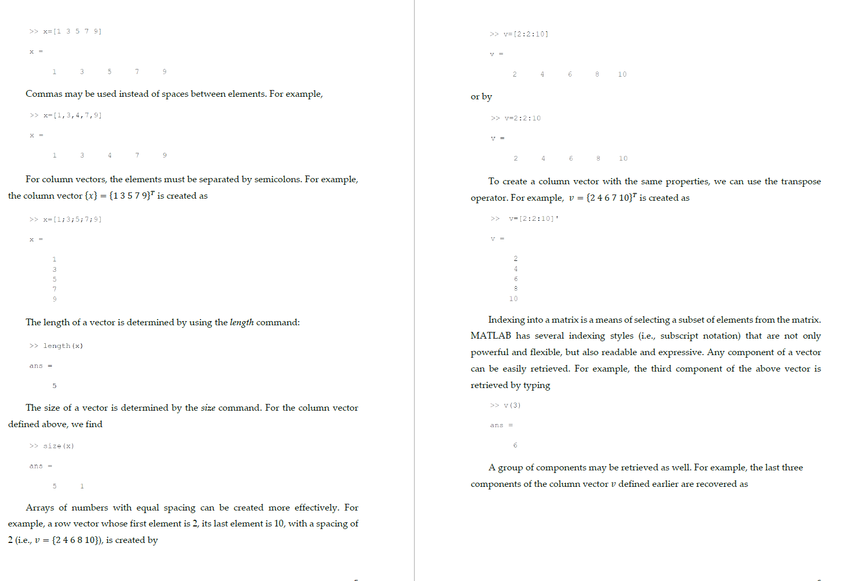
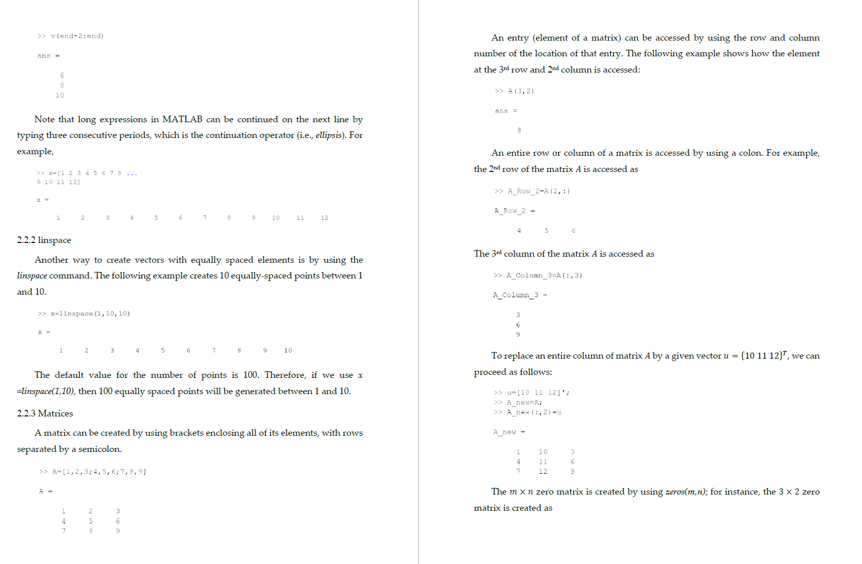
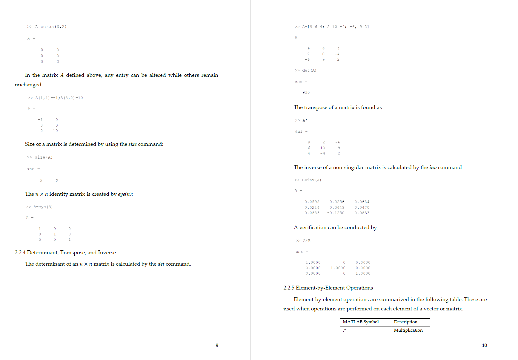
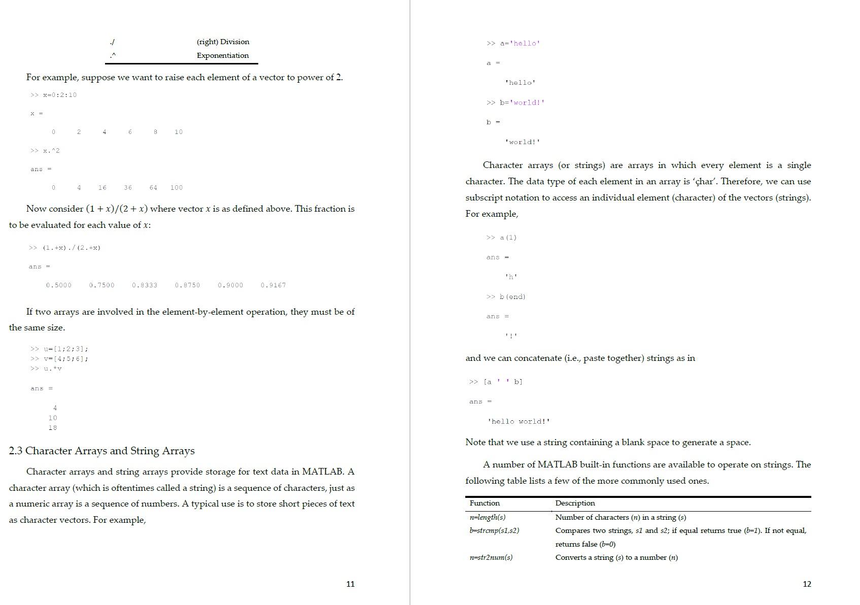
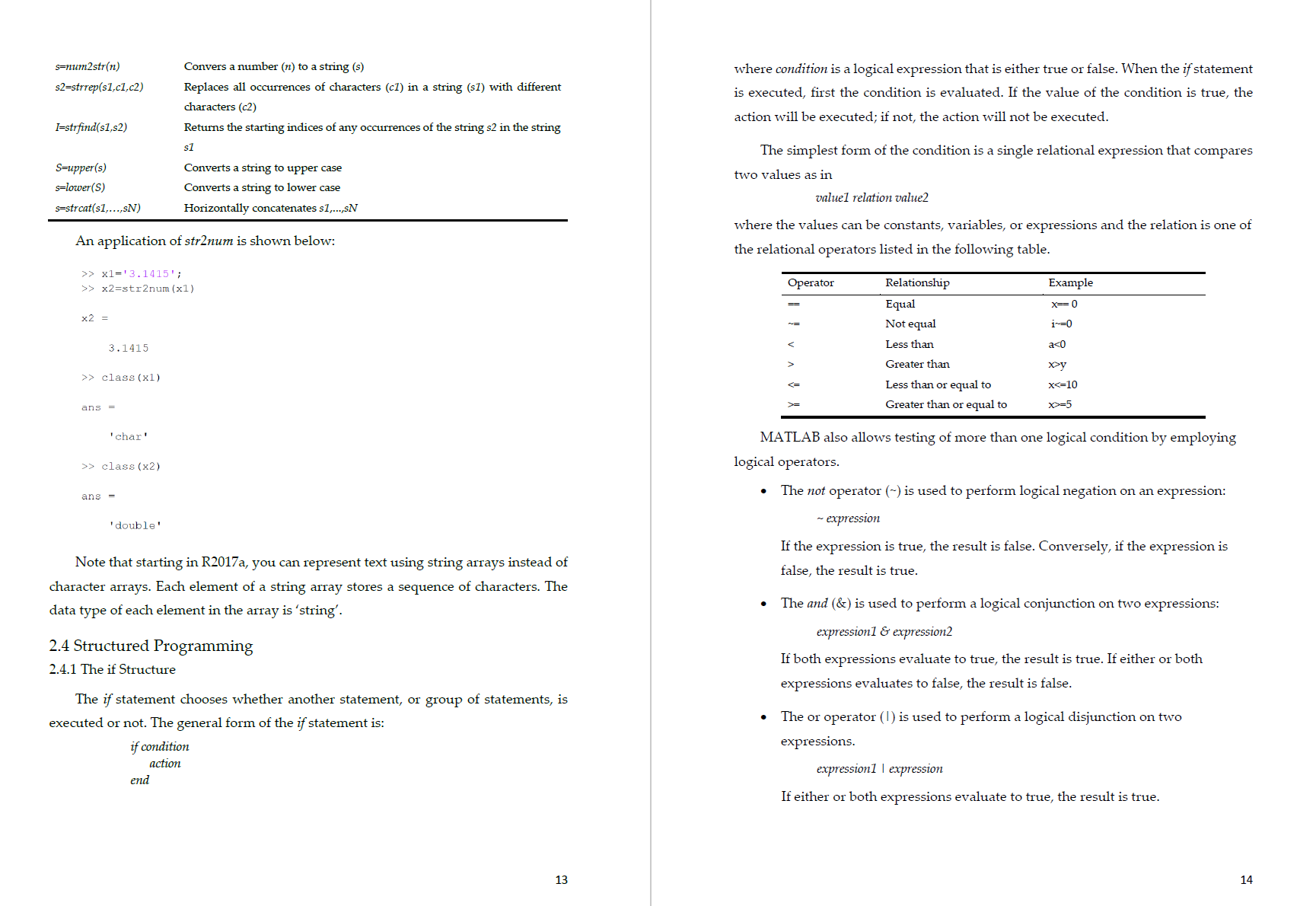
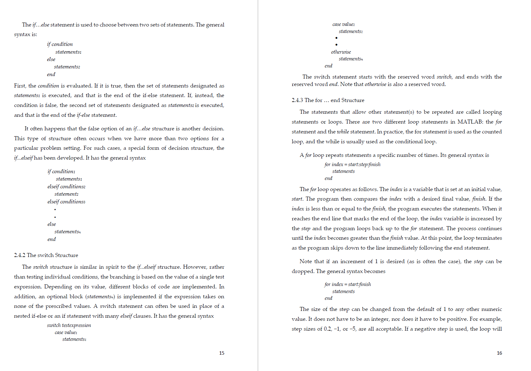
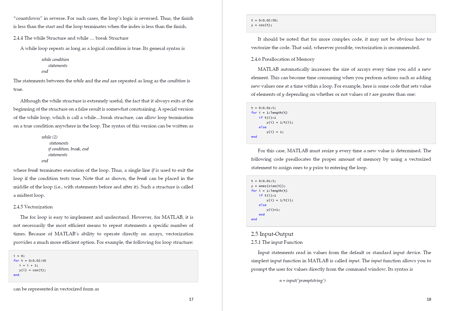
\fThe function displays the promptstring, waits for keyboard input, and then returns the value from the keyboard. For example, >> velocityZlnput('Ve_ c".:; (mm; ') Velocity (In/B): 50.6175 velocity = 50.6175 In this example, the value of user input is assigned to the variable velocity. The input function can also return user input as a string. To do this, an 's' is appended to the function's argument list. For example, >> Lette::input('Enr=.-; e, Chadet-er: '."a't Enter a character: a letter = .5. 2.5.2 The disp Function Output statements display strings andlor the results of expressions, and may allow for formatting or customin'ng how they are displayed. The simplest output mction in MATLAB is disp with the following syntax dispfmluel Where value = the value you would like to display. It can be a numeric constant or variable, or a string message enclosed in hyphens. However, the disp function does not allow formatting. For example, >> disp( 'hE-llL' wo:l_d l ' l hello World! >> disptpil 3.1416 2.5.3 The fprint'f Function Formatted output can be printed to the screen or written to a file using the fprintf function. A simple representation of its syntax is nint'lnnt', 1,...) for output to the screen, or fprintd, 'fmma't', I, ...) 19 for output to a le with a le identifier li. The format is a string specifying how you want the value of the variable x to be displayed. Commonly used format and control oodes employed with the fprmtf function are listed in the following table. Formal Code Description std Integer lei-mat 9&2 Scientic format with lowerrase e 'BBE Scientic format with uppercase E '3\" Deunlal (mt 'tbg The mm compact of 96a and 'M Control Code Description \ Start new line \\t Tab A field width can also be included in the place holder in fprmtf, which species how many characters in total are to be used in printing. For example, 965:} would indicate a eld width of 5 for printing an integer and "12103 would indicate a field width of 10 for a string. For oats, the number of decimal places can also be specified; for example, %6.2fmeans a field width of 6 (including the decimal point and the two decimal places) with 2 decimal plaoes. For oats, just the number of decimal places can be specied; for example, %.3f indicates 3 decimal places, regardless of the field width. A simple example would he to display a value along with a message. For instanoe, suppose that the variable velocity has a value of 50.6175. To display the value using eight digits with four digits to the right of the decimal point along with a message, the statement along with the resulting output would be >2 velocuyusns; > {pagan-1 .- (-l u, i ~h;-_"1' velocity) The Velocity L5 50.6175 III/s This example illustrates how the format string works. MATLAB starts at the left end of the string and displays the labels until it detects one of the symbols: % or \\. In the example, it rst encounters a /u and recognizes that the following text is a format 20 \fcode. The format codes allow you to specify whether numeric values are displayed in integer, decimal, or scientific format. In this example, \"/uSAf indicates the velocity value is outputted in a format of a field width of 8 with 4 decimal places. After displaying the value of velocity, MATLAB continues displaying the character information (in the case the units: m/s) until it detects the symbol \\. This tells MATLAB that the following text is a control code. The control codes provide a means to perform actions such as skipping to the next line. If we had omitted the code \ in the previous example, the command prompt would appear at the end of the label m/s rather than on the next line as would typically be desired. 2.5.4 Create and Access Files Using save and load Functions MATLAB has the capability to both read and write data files. The simplest approach involves a special type of binary file, called a MATefile, which is expressly designed for implementation within MATLAB. Such tiles are created and accessed with the save and load commands. The save command can be used to generate a MATefile holding either the entire workspace or a few selected variables. A simple representation of its syntax is smlemm: mm van van 'scii' This command creates a MATifile named lemrmemmt that holds the variables mm through our". If the variables are omitted, all the workspace variables are saved. The "fascii\" qualier is used when creating a text or data file. The load command can subsequently be used to retrieve the file: loadlcmzme van W2 mm asco" which retrieves the variables For] through mm. fromlename.mat. As was the case with save, if the variables are omitted, all the variables in the workspace are retrieved. The following example illustrates how a randomly generated 2 X 3 matrix is saved to a data le and loaded to the Workplace from the saved file. 21 >> myrnat=rendt4r3l mymat = 0.5943 0.4337 0.1369 0.3171 0.3816 0.4998 0.9502 0.7655 0.4456 0.0344 0.7952 0.6463 >> save rs file.dar mymar '7asc:i' >> clear m >> type :2 f11e,det 6.9482362e-l .38744365-01 3.170994Berl .E155846erl 4 .BGSTZEOe-Ol 3 9.5022205e-Ul 7.655167De-01 7 at .8976440erl .ajSBszOeol .46313015701 mun-DH 3.4446091e702 .9519; 701 >> load teatfile.d 'reac >> who Your variables are: testfile >> testfile testfile = 0.5943 0.4337 0,1569 0.3171 0.3816 0.4598 0.9502 0.7655 0.4456 0.0344 0.7952 0.6463 As demonstrated in the example, the type command can be used to display the contents of the file; note that scientific notation is used. Once a le has been created, it can be read into a matrix variable. [fthe file is a data file, the load command will read from the le \"lenameex't" (e.g. the extension might be .dat) and create a matrix with the same name as the file. In the above example, the data le \"testliile.dat" was created, the load command read from it, and stored the result in a matrix variable called testle. Alternatively, you oould use the load command as a function and assign its Values to a variable as in 22 >> B:load('testf;le.dat') a: 0.6948 DASH? 0.1869 0.3171 0.38.16 0.4896 0.9502 0.7655 0.4456 0.0344 0.7952 0.6463 The load command works only if there are the same number of values in each line, so lat the data can be stored in a matrix, and the save command only writes from a matrix to a le. 2.5.5 LowerLevel File l/O Functions When writing to and reading from a data file, the save and load function works as long as the data in the le are "regular" structured in form of a matrix, that is, the same kind of data on every line and in the same format on every line. When it is not possible to use load, MATLAB has what are called lowerelevel file input functions lat can be used. The file must be opened rst, which involves finding or creating the le and positioning an indicator at the beginning of the file. This indicator then moves through the le as it is being read from or written to. When the reading or writing has been completed, the le must be closed. In general, le steps involved are: I open the file I read from the le, write to le le, or append to the file I close le le Files are opened with the foperr function. The general form is d :rpmlemme, 'pemussiml string? Whered is a variable that stores the le identifier (it can be named anything) and the 'permissm strings' include: '1' Open tile for reading. 'w' Open or create new le for writing. Discard existing contents, it any. 'a' Open or create new le for writing. Append data to the end of the tile. After the fapen is attempted, the value returned should be tested to make sure that the le was opened successfully. For example, if attempting to open for reading and the file does not exist, the fopen will not be successful. As the fapen function returns ,1 23 if the file was not found, this can be tested to decide whether to print an error message or to carry on and use the file. Files should be closed when the program has finished reading from or writing or appending to them. The function that accomplishes this is the fclnse function, which returns 0 if the file close was successful or 71 if not. Individual files can be closed by specifying the file identier. The general forms are: closerESlllt : fclosel'd) The result from the fclose function should also be checked with an ifielse statement to make sure it was successful, and a message should be printed. The outline of the code is given below: d :ipenffilenm', permission string' J; ifd : *1 dispfle open not successful') else % do smnething with thele! cIaserzsult :fclosetd); Ifcloseresult = 0 dispfFiie ClSE successll') else dis 'Fik dose not successrl') end end There are several lower-level functions that read from files. The fgetl and fgets functions read strings from a file one line at a time; the difference is that thefgets keeps the newline character if there is one at le end of the line, whereas the fgel'l function gets rid of it. Both of these functions require first opening the file, and len closing it when finished. The fgefl function reads one line of data from a file into a string; string functions can len be used to manipulate the data. As fgetl only reads one line, it is normally placed in a loop lat keeps going until the end of the file is reached. The functionfeuf returns logical true if the end of the file has been reached. The function call feod) would return logical true if the end of the file has been reached for the file identified byd, or logical false if not. A general algorithm for reading from a file into strings would be: d = fopmt lmm'); 24 \f\f\f:>> d:TestFuncScCIIe (x, y) 10 if: 15 If we type in the command window to request output of c, x, and a, we obtain >> c, x, a c: 10 UnLecagnLZed function or variable 'a'. >> The point here is that even though I was assigned a new value inside the function, the variable of the same name in the MATLAB workspace is unchanged. Even though they have the same name, the scope of each is liJnited to their oontext and does not overlap. In the function, the variables :1 and b are limited in soope to that function, and only exist while that function is being executed. Such variables are formally called local variables. Thus, when we try to display the Value of a in the workspaoe, an error message is generated because the workspace has no access to the a in the function. The function's argument list is like a window through which information is selectively passed between the workspaoe and a function, or between two functions. Sometimes, however, it Inight be convenient to have access to a variable in several 31 contexts without passing it as an argument. In such cases, this can be acoomplished by defining the variable as global. This is done with the global command, which is dened as glbl mnblefs) where the variables (e.g., X, Y, Z) dened in the variables list are global in scope. If several functions all dechre a particular name as global, then they all share a single value of that variable. Any change to that variable, in any function, is then made to all the other functions that declare it global. stylistically, MATLAB reoommends that global variables use all capital letters, but this is not required. 2.6.4 Anonymous Functions An anonymous function is a simple, onerline function. The advantage of an anonymous function is that it does not have to be stored in a separate Mele. They can be defined within the command window or in an existing Mele with the following syntax: landlz = @(arglisl) expression whereumdle : the function handle you can use to invoke the function, it is essentially a Way of referring to the function; arglist : a conuna separated list of input arguments in parentheses to be passed to the function; and expression : any single valid MATLAB expression For example, >9 fun:@tx,yl whys >,~ funl3.43 ans : 25 2.6.5 Function Functions Function functions are functions that operate on other functions which are passed to it as input arguments. One reason for using function handles is to be able to pass functions to function functions. MA'ILAB has some builtrin function functions. The function function ferret will evaluate a function handle and execute the function for the speded argun1ent. For example: 32 \f[n the above gure, labels are put on the x-axis, the y-axis, and the graph itsell 2_8 Examples using the functions xlabel, global, and title. The axis limits are specified by using the 2,8,1 Calculate roots of a quadratic equation axistlimits) command, in which limits is a vector to limit the axis range. For the 2D Given a general quadratic equation of the form plot, the first two values are the minimum and maximum for the x-axis, and the last 75 : ax2 + bx + c two are the minimum and maximum for the yeaxis. fl: ) with 1: representing an unknown, :1, b and C representing constants with a s5 0, the The followmg example illustrates how to specily line style, color and marker in the quadratic formula is: plat command. The example plots three sine curves with a small phase shift between each line. The specification uses a green Line with no markers for the first sine curve; I 7 *b i #112 7 4m: 7 211 uses a blue dashed line with circle markers for the second sine curve; and uses only k f th third , If the constant a = 0, there is a single real root: x = 76/11. cyan star mar ers or e sine curve. In the quadratic formula, the expression underneath the square root sign is called x=n=pI/10=Z*p1: the discriminant of the quadratic equation: y n(x): y n(Xr0.25); Y3:s1n(x-0.5]: A : b2 4'15 p1nt(x.y1.'g' ,xgv2.'h"> x=[l, 3,4,7,9] x= For column vectors, the elements must be separated by semicolons. For example, the column vector {x} : {1 3 5 7 9}T is created as >> x:[.;3;.w;i] wlmmbd m The length of a Vector is determined by using the length command: >> length (x) 61115 = The size of a vector is determined by the size command. For the colunln vector dened above, we find >> 5129 (x) Arrays of numbers with equal spacing can he created more effectively. For example, a row vector whose first element is 2, its last element is 10, with a spacing of 2 (ie., I) = {Z 4 6 8 10)), is created by ,~:= v=[2:2:10] or by >> V:2:2:lU 2 4 E B :D To create a column vector with the same properties, we can use the transpose operator. For example, I) = {2 4 6 7 10V is created as >> V=[2:2:10" Indexing into a matrixis ameans of selecting a subset of elements from the matrix. MATLAB has several indexing styles (i.e., subscript notation) that are not only powerful and exible, but also readable and expressive. Any oomponent of a vector can be easily retrieved. For example, the third component of the above vector is retrieved by typing >> v (31 ans 7 A group of oomponents may be retrieved as well. For exalnple, the last three components of the colunm vector I) defined earlier are recovered as >5 v(end*2:end) Note that long expressions in MATLAB can be conrmed on the next line by typing three consecutive periods, which is the continuation operator (i.e., ellipsis). For example, :.>x=[:234557a Q 10 l: 12] x = 1 z 3 1 s e 7 e u 10 11 12 2.2.2ljnspace Another way to create vectors with equally spaced elements is by using the limpace command. The following example creates 10 equallyispaced points between 1 and 10. >> X=lrnspaee(l,10, 10) The default value for the number of points is 100. Therefore, if we use a: impacd 1,10), then 100 equally spaced points will be generated between 1 and 10. 2.2.3 Matrices A matrix can be created by using brackets enclosing all of its elements, with rows separated by a semicolon. >> A=[l,2,3;4,5,6;7,8.9l p= l 2 3 4 5 6 7 E 9 An entry (element of a matrix) can be accessed by using the row and column number of the location of that entry. The following example shows how the element at the 3" row and 2nd column is accessed: >> 3.13.21 ans 7 a:- An entire row or column of a matrix is accessed by using a colon. For example, the 2"\" row of the matrix A is accessed as >> P7Hoh172=l (2, :x The 31\" column of the matrix A is accessed as >> A_Cnlumn_3=A(: ,3} A7Column73 : 3 6 9 To replace an entire column of matrix A by a given vector u = {10 11 12?, we can proceed as follows: >) u=[lC' ll 12]'; >> A:newt:,2)=J Ainew = 'l l D 3 4 1 l. 6 '7 1.2 9 The m X 11 zero matrix is created by using zms(m,n); for instance, the 3 x 2 zero matrix is created as \f./ (nght)D1visiun >> a= ' mum .A FJcponenuatiun For example, suppose We want to raise each element of a vector to power of 2. 'halla' >> x=u:2:13 >> b:'wUIldl' x : h = u z 4 6 8 1C 'wnrld.' ' u x.\"2 ans = Character arrays (or strings) are arrays in which every element is a single n 4 _ 6 36 1 10D character. The data type of each element in an array is l> 3(1) >> (1.+x).f2.+xb an? = an: = .J' c.50u3 3.7500 0.3353 imam 0.9m: D.91E1 hIend] If two arrays are involved in the elementihyelement operation, they must be of _ ans _ thesame size. Hi >> r.= l;2;3]; 4 i 5 .- a] ; and we can concatenate (i_e., paste together) strings as in >> L.'V >> [a ' ' b] ans = ans = 4 1" 'hello world!' is Note that we use a string containing a blank space to generate a space. 2.3 Character Arrays and String Arrays A number of MATLAB builtein functions are available to operate on strings. The Character arrays and string arrays provide storage for text data in MATLAB. A . . _ _ _ _ following table lists a few of the more commonly used ones. character array (which is oftentimes called a stung) Is a sequence of characters, lust as a numeric array is a sequence of numbers. A typical use is to store short pieces of text Function Description as character vectors. For example, ngthfs) N'm'be' 0' \"m5 ('0 in am (5) Lemmpersu Compares two strings, 51 and 52,- 1 equal returns true (b4). If not equal, returns false (b=0) Panama) Converts a string (5) to a nuinbet (n) 11 12 Fumzshw Convers a number (n) to a suing (s) shtneptsrmrcz) Replaces all oocunenoes of characters (:1) in a string (51) with Meat characters (:2) I=sirndsts2l Returns the starting inclines of any occurrences of the string 52 in the string 51 Wrens) Converts a string to upper case FMS) Converts a string to lower case stslp . .,sN) Horizontally cancaterlates sI,...,5N An application of stanum is shown below: >> x1: lilillS'y' >> x23tanum(x1) x2 : 3,1415 >> aiaaazxu ans 7 'char' >> classtth ens = 'double ' Note that starting in R2017a, you can represent text using string arrays instead of character arrays. Each element of a string array stores a sequence of characters. The data type of each element in the array is 'stn'ng'. 2.4 Structured Programming 2.4.1 The ii Structure The if statement chooses whether another statement, or group of statements, is executed or not. The general form of the If statement is: if condition action and 13 where condition is a logical expression that is either true or false. When the lfstatement is executed, first the condition is evaluated. It the value of the condition is true, the action will be executed; if not, the action will not be executed. The simplest form of the condition is a single relational expression that compares two values as in value] relaiiml value? where the values can be constants, Variables, or expressions and the relation is one of the relational operators listed in the following table. Operator Relationship Brample = Equal x: 0 77 Nm equal i~=a Greater than x>y : Greater than or equal to x>z5 MATLAB also allows testing of more than one logical condition by employing logical operators. I The not operator (~) is used to perform logical negation on an expression: N WESSIO'II ll the expression is true, the result is false. Conversely, if the expression is false, the result is true. I The and (Sr) is used to perform a logical conjunction on two expressions: expressianl 8 mressilmz ll both expressions evaluate to true, the result is true. If either or both expressions evaluates to false, the result is false. - The or operator (I) is used to perfonn a logical disjunction on two expressions. expression] l expression If either or both expressions evaluate to true, the result is true. 14 The if. . .2192 statement is used to choose between two sets of statements. The general syntax is: if condition stotementsi etse statementsz and First, the condition is evaluated. If it is true, then the set of statements designated as statements; is executed, and that is the end of the ifelse statement. If, instead, the condition is false, the second set of statements designated as statementsz is executed, and that is the end of the ifflse statement. It often happens that the false option of an if. . .else structure is another decision. This type of structure often occurs when we have more than two options for a particular problem setting. For such cases, a special form of decision structure, the fuelseifhas been developed. It has the general syntax ifconditionr statements: elseifeonditionsz statementz elseifeonditimisa else statementSn end 3.4.2 The switch Structure The switch structure is similar in spirit to the if...etse# structure. However, rather than testing individual conditions, the branching is based on the Value of a single test expression. Depending on its value, different blocks of code are implemented. In addition, an optional block (statemmtSn) is implemented if the expression takes on none of the prescribed values. A switch statement can often be used in place of a nested iLelse or an if statement with many elseif clauses. It has the general syntax switch testexpressian ease value; statements: 15 case value: statements: otherwise statementsK end The switch statement starts with the reserved word switch, and ends with the reserved Word end. Note that otherwise is also a reserved word. 2.4.3 The for end Structure The statements that allow other statement(s) to be repeated are called looping statements or loops. There are two different loop statements in MA'TLAB: the for statement and the while statement. In practice, the for statement is used as the counted loop, and the while is usually used as the conditional loop. Afar loop repeats statements a specific number of times. Its general syntax is n index : startstepnlsh statements end The for loop operates as follows. The index is a variable that is set at an initial value, start. The program then compares the index with a desired final value, nish. If the index is less than or equal to the nish, the program executes the statements. When it reaches the end Line that marks the end of the loop, the index variable is increased by the step and the program loops back up to the for statement. The process continues until the index becomes greater than the nish Value. At this point, the loop terminates as the program skips down to the Line immediately following the end statement. Note that if an increment of 1 is desired (as is often the case), the step can be dropped. The general syntax becomes formdex=stm:nish statements end The size of the step can be changed from the default of l to any other numeric value. It does not have to be an integer, nor does it have to be positive. For example, step sizes of 0.2, *1, or *5, are all acceptable. If a negative step is used, the loop will 16 \"countdown" in reverse. For such cases, the loop's logic is reversed. Thus, the finish is less than the start and the loop terminates when the index is less than the finish. 2.4.4 The white Structure and while break Structure A while loop repeats as long as a logical condition is true. Its general syntax is while condition statements and The statements between the while and the emf are repeated as long as the condition is true. Although the while structure is extremely useful, the fact that it always exits at the beginning of the structure on a false result is somewhat constraining. A special version of the while loop, which is call a While...break structure, can allow loop termination on a true condition anywhere in the loop. The syntax of this Version can be written as while (I) statements If condition, hulk, end statements end where break terminates execution of the loop. Thus, a single line If is used to exit the loop if the condition tests true. Note that as shown, the break can be placed in the middle of the loop (i.e., with statements before and after it). Such a structure is called a midtest loop. 2.4.5 Vectorization The for loop is easy to implement and understand. However, for MATLAB, it is not necessarily the most efficient means to repeat statements a specific number of times. Because of MATLAB's ability to operate directly on arrays, vectorization provides a much more efcient option. For example, the following for loop structure: 1 : u; for t = :.02:50 i w- 1; y(1') = custtl: end can he represented in Vectorized form as 17 o: n . 02 : so; (05(t); It should he noted that for more complex code, it may not be obvious how to vectorize the code. That said, wherever possible, vectorization is recommended. 2.4.6 Preallocation of Memory MATLAB automatically increases the size of arrays every time you add a new element. This can become time consuming when you perform actions such as adding new values one at a time within a loop. For example, here is some code that sets value of elements of 3; depending on Whether or not Values oft are greater than one: 1 : o:n.or:5: inangmrt) if t(i)>1 vh) = 11th): else VG) = 1: for 1' end For this case, MATLAB must resize y every time a new value is determined. The following code preallocates the proper amount of memory by using a vectorized statement to assign ones to y prior to entering the loop. 1 = o:n.or:s; ones (51 2e (t)) ; 1' : 1:1:ng-[D if t(i)>1 vh) = 1/t(i): else y(1)=1; end (ml 2.5 InputOutput 2.5.1 The input Function Input statements read in values from the default or standard input device. The simplest input function in MATLAB is called input. The input function allows you to prompt the user for values directly from the command Window. Its syntax is n : inpu 'pmmpistring') 18