ANSWERS FOR THE YELLOW BOXES BELOW MUST BE SHOW BASED ON FUNCTIONS DOWN BELOW
EXAMPLE "=C7" OR "=SUM(C7,C9)"


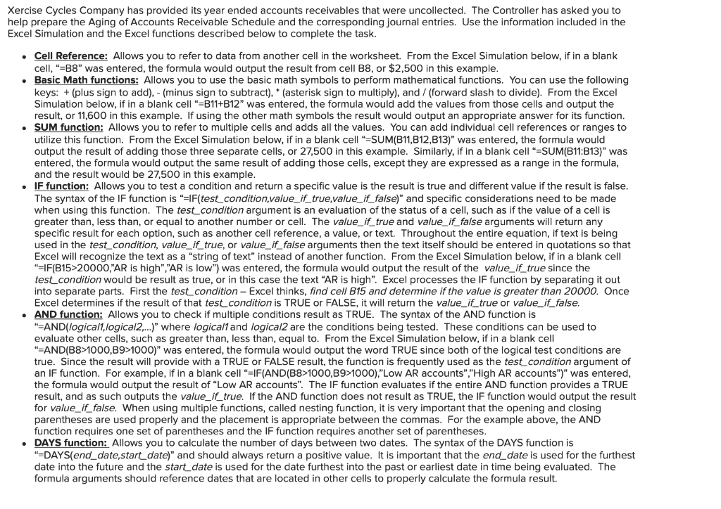
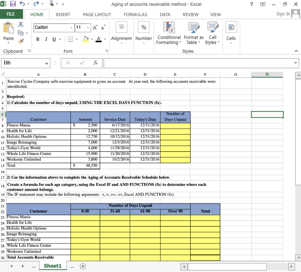
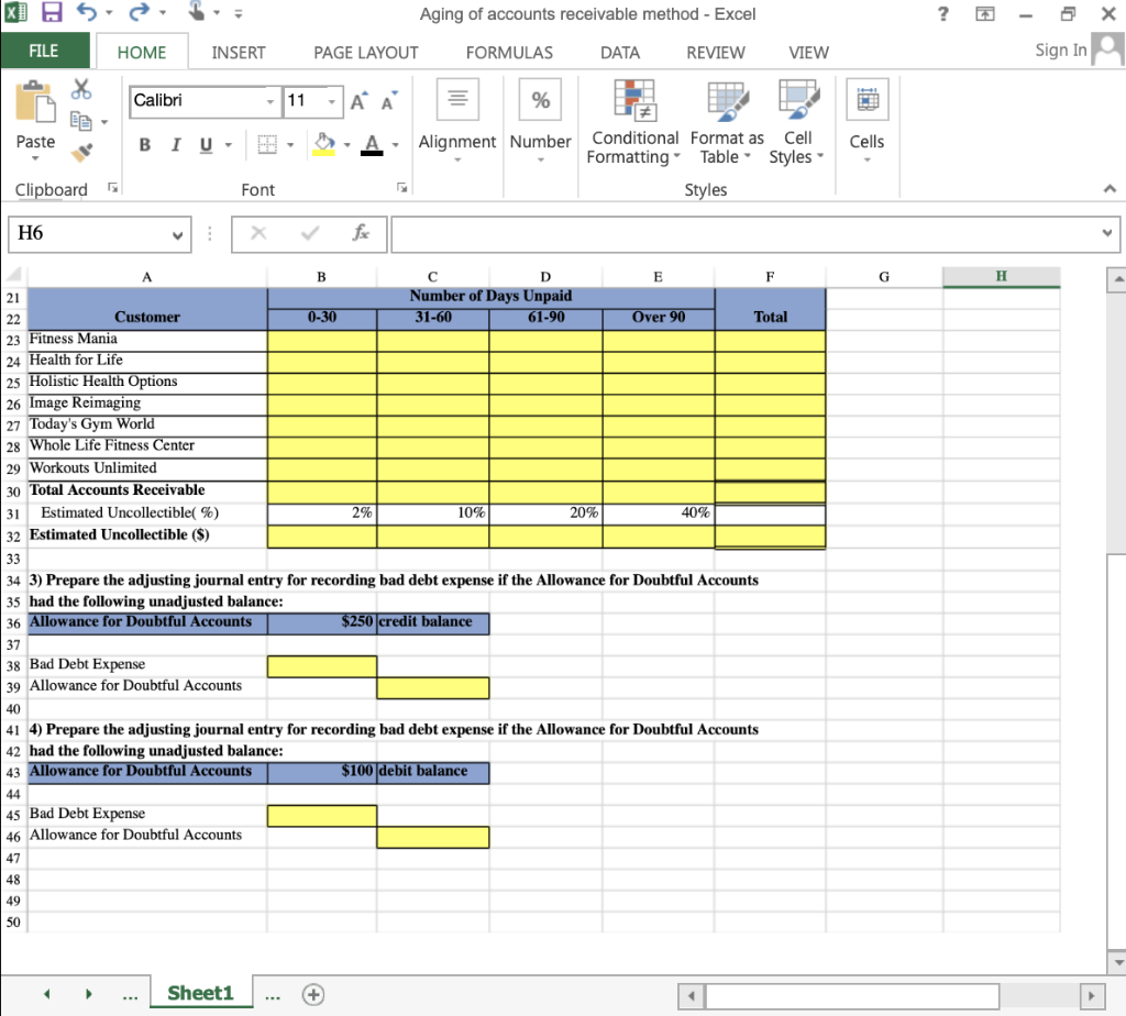
Xercise Cycles Company has provided its year ended accounts receivables that were uncollected. The Controller has asked you to help prepare the Aging of Accounts Receivable Schedule and the corresponding journal entries. Use the information included in the Excel Simulation and the Excel functions described below to complete the task. Cell Reference: Allows you to refer to data from another cell in the worksheet. From the Excel Simulation below, if in a blank cell, =B8" was entered, the formula would output the result from cell B8, or $2,500 in this example. Basic Math functions: Allows you to use the basic math symbols to perform mathematical functions. You can use the following keys: + (plus sign to add), - (minus sign to subtract), * (asterisk sign to multiply), and / (forward slash to divide). From the Excel Simulation below, if in a blank cell "=B11+B12" was entered, the formula would add the values from those cells and output the result, or 11,600 in this example. If using the other math symbols the result would output an appropriate answer for its function. SUM function: Allows you to refer to multiple cells and adds all the values. You can add individual cell references or ranges to utilize this function. From the Excel Simulation below, if in a blank cell"=SUM(B11,B12,813)" was entered, the formula would output the result of adding those three separate cells, or 27,500 in this example. Similarly, if in a blank cell"=SUM(B11:B13)" was entered, the formula would output the same result of adding those cells, except they are expressed as a range in the formula, and the result would be 27,500 in this example. IF function: Allows you to test a condition and return a specific value is the result is true and different value if the result is false. The syntax of the IF function is "=IF(test_condition, value_if_true,value_if_false)" and specific considerations need to be made when using this function. The test_condition argument is an evaluation of the status of a cell, such as if the value of a cell is greater than, less than or equal to another number or cell. The value_if_true and value_if_false arguments will return any specific result for each option, such as another cell reference, a value, or text. Throughout the entire equation, if text is being used in the test_condition, value_if_true, or value_if_false arguments then the text itself should be entered in quotations so that Excel will recognize the text as a string of text" instead of another function. From the Excel Simulation below, if in a blank cell "=IF(815>20000,"AR is high","AR is low") was entered, the formula would output the result of the value_if_true since the test_condition would be result as true, or in this case the text AR is high". Excel processes the IF function by separating it out into separate parts. First the test_condition - Excel thinks, find cell B15 and determine if the value is greater than 20000. Once Excel determines if the result of that test_condition is TRUE or FALSE, it will return the value_if_true or value_if_false. AND function: Allows you to check if multiple conditions result as TRUE. The syntax of the AND function is "=AND(logical1,logical2...)" where logical and logical2 are the conditions being tested. These conditions can be used to evaluate other cells, such as greater than, less than, equal to. From the Excel Simulation below, if in a blank cell "=AND(B8>1000,89>1000)" was entered, the formula would output the word TRUE since both of the logical test conditions are true. Since the result will provide with a TRUE or FALSE result, the function is frequently used as the test_condition argument of an IF function. For example, if in a blank cell =IF(AND(B8>1000,09>1000),"Low AR accounts,"High AR accounts")" was entered, the formula would output the result of Low AR accounts". The IF function evaluates if the entire AND function provides a TRUE result, and as such outputs the value_if_true. If the AND function does not result as TRUE, the IF function would output the result for value_if_false. When using multiple functions, called nesting function, it is very important that the opening and closing parentheses are used properly and the placement is appropriate between the commas. For the example above, the AND function requires one set of parentheses and the IF function requires another set of parentheses. DAYS function: Allows you to calculate the number of days between two dates. The syntax of the DAYS function is "=DAYS(end_date,start_date)" and should always return a positive value. It is important that the end_date is used for the furthest date into the future and the start date is used for the date furthest into the past or earliest date in time being evaluated. The formula arguments should reference dates that are located in other cells to properly calculate the formula result X] 5 Aging of accounts receivable method - Excel ? X FILE HOME INSERT PAGE LAYOUT FORMULAS DATA REVIEW VIEW Sign In Calibri 11 AA % DE Paste BIU- A- Alignment Number Cells Conditional Format as Cell Formatting Table Styles Styles Clipboard Font H6 V fx A B D F G H E Xercise Cycles Company sells exercise equipment to gyms on account. At year end, the following accounts receivable were uncollected. 1 3 Required: 4 1) Calculate the number of days unpaid, USING THE EXCEL DAYS FUNCTION (fx). 5 6 Number of 7 Customer Amount Invoice Date Today's Date Days Unpaid 8 Fitness Mania S 2,500 6/17/2016 12/31/2016 9 Health for Life 2.000 12/21/2016 12/31/2016 10 Holistic Health Options 12,750 10/12/2016 12/31/2016 11 Image Reimaging 7,000 12/5/2016 12/31/2016 12 Today's Gym World 4,600 11/29/2016) 12/31/2016 13 Whole Life Fitness Center 15.900 11/20/2016 12/31/2016 14 Workouts Unlimited 3,800 10/2/2016 12/31/2016 15 Total $ 48.550 16 17 2) Use the information above to complete the Aging of Accounts Receivable Schedule below. 18 Create a formula for each age category, using the Excel IF and AND FUNCTIONS (fx) to determine where each customer amount belongs. 19 The IF statement may include the following arguments: , >=, Sheet1 + Aging of accounts receivable method - Excel ? 6 X FILE HOME INSERT PAGE LAYOUT FORMULAS DATA REVIEW VIEW Sign In Calibri 11 - A % Paste BIU A- Cells Cell Alignment Number Conditional Format as Formatting Table Styles Styles Clipboard Font A H6 face V H A B C D E F 21 Number of Days Unpaid 22 Customer 0-30 31-60 61.90 Over 90 Total 23 Fitness Mania 24 Health for Life 25 Holistic Health Options 26 Image Reimaging 27 Today's Gym World 28 Whole Life Fitness Center 29 Workouts Unlimited 30 Total Accounts Receivable 31 Estimated Uncollectible(%) 2% 10% 20% 40% 32 Estimated Uncollectible ($) 33 34 3) Prepare the adjusting journal entry for recording bad debt expense if the Allowance for Doubtful Accounts 35 had the following unadjusted balance: 36 Allowance for Doubtful Accounts $250 credit balance 37 38 Bad Debt Expense 39 Allowance for Doubtful Accounts 40 41 4) Prepare the adjusting journal entry for recording bad debt expense if the Allowance for Doubtful Accounts 42 had the following unadjusted balance: 43 Allowance for Doubtful Accounts $100 debit balance 44 45 Bad Debt Expense 46 Allowance for Doubtful Accounts 47 48 49 50 Sheet1 +
