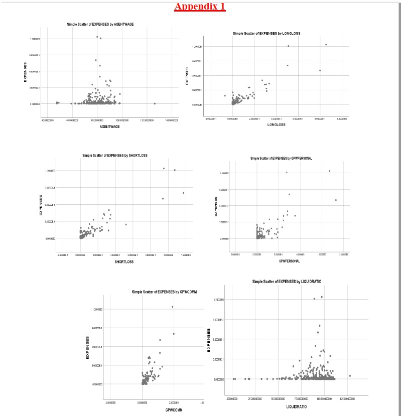
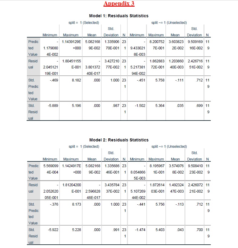
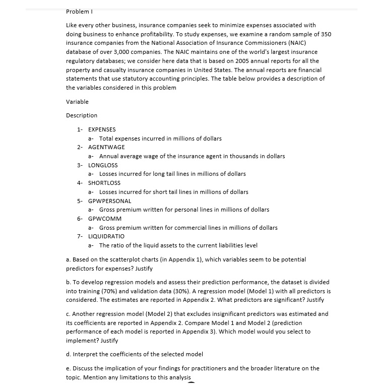
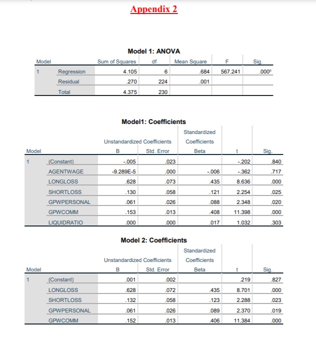
Appendix 1 Simple Scatter of EXPENSES by AGENTWAGE Simple Scatter of EXPENSES by LONGLOSE EXPENSES EXPENSE AGENTWAGE LONGLOSS Simple Scatter of EXPENSES by SHORTLOSS Simple Souther of EXPENSES by GPWPERSONAL EXPONECE EXPENSES SHORTLOSS SPINPERSONAL Simple Scatter of EXPENSES by LIQUIDRATIO Simple Scatter of EXPENSES by GPWCOMM EXPENSE EXPENSE DOOLDEN 135 00800100 GPWCOMM LIQUIDRATIOAppendix 2 Model 1: ANOVA Model Sum of Squares dif Mean Square F Sig Regression 4.105 6 684 567.241 000- Residual .270 224 001 Total 4.375 230 Model1: Coefficients Standardized Unstandardized Coefficients Coefficients Model B Std. Error Beta Sig (Constant) -.005 023 -.202 840 AGENTWAGE -9.289E-5 000 .006 -.362 717 LONGLOSS 628 073 435 8.636 000 SHORTLOSS 130 058 121 2.254 .025 GPWPERSONAL 061 026 088 2.348 020 GPWCOMM .153 013 408 11.398 000 LIQUIDRATIO .000 .000 017 1.032 303 Model 2: Coefficients Standardized Unstandardized Coefficients Coefficients Model B Std. Error Beta Sig (Constant) 001 002 219 827 LONGLOSS 628 072 435 8.701 000 SHORTLOSS 132 058 123 2.288 023 GPWPERSONAL 061 026 089 2.370 019 GPWCOMM 152 013 406 11.384 000Appendix 3 Model 1: Residuals Statistics split = 1 (Selected) split ~= 1 (Unselected) Std. Std Minimum Maximum Mean Deviation N Minimum Maximum Mean Deviation N Predic 1.1439129E 5.082168 1.335906 23 8.200752 3.603823 9.509169 11 ted 1.179080 +000 9E-002 70E-001 1 9.433021 7E-001 2E-002 16E-002 9 Value 4E-002 8E-003 Resid 1.80451155 3.427210 23 1.862883 1.203860 2.426716 11 ual 2.045121 E-001 3.801372 77E-002 5.217381 72E-001 40E-003 51E-002 19E-001 40E-017 94E-002 Std. -.469 8.182 000 1.000 23 .451 5.758 -.111 712 11 Predic ted Value Std. 5.889 5.196 000 987 23 -1.502 5.364 .035 699 11 Resid 9 ual Model 2: Residuals Statistics split = 1 (Selected) split ~= 1 (Unselected) Std. Std Minimum Maximum Mean Deviation N Minimum Maximum Mean Deviation IN Predic 5.569099 1.14249178 5.082168 1.335686 23 8. 195967 3.574976 9.508410 11 ted 4E-004 +000 9E-002 46E-001 1 8.054866 1E-001 BE-002 23E-002 9 Value 5E-003 Resid 1.81204200 3.435784 23 1.872614 1.492324 2.426072 11 val 2.052620 E-001 2.596828 37E-002 5.107269 03E-001 47E-003 21E-002 05E-001 48E-017 44E-002 Std. -.376 8.173 .000 1.000 23 -.441 5.756 .113 712 11 Predic ted Value Std. -5.922 5.228 .000 .991 23 -1.474 5.403 043 .700 11 Resid ualProblem I Like every other business, insurance companies seek to minimize expenses associated with doing business to enhance profitability. To study expenses, we examine a random sample of 350 insurance companies from the National Association of Insurance Commissioners (NAIC) database of over 3,000 companies. The NAIC maintains one of the world's largest insurance regulatory databases; we consider here data that is based on 2005 annual reports for all the property and casualty insurance companies in United States. The annual reports are financial statements that use statutory accounting principles. The table below provides a description of the variables considered in this problem Variable Description 1- EXPENSES a- Total expenses incurred in millions of dollars 2- AGENTWAGE a- Annual average wage of the insurance agent in thousands in dollars - LONGLOSS a- Losses incurred for long tail lines in millions of dollars SHORTLOSS a- Losses incurred for short tail lines in millions of dollars 5 - GPWPERSONAL a- Gross premium written for personal lines in millions of dollars 6- GPWCOMM a- Gross premium written for commercial lines in millions of dollars 7- LIQUIDRATIO a- The ratio of the liquid assets to the current liabilities level a. Based on the scatterplot charts (in Appendix 1), which variables seem to be potential predictors for expenses? Justify b. To develop regression models and assess their prediction performance, the dataset is divided into training (70%) and validation data (30%). A regression model (Model 1) with all predictors is considered. The estimates are reported in Appendix 2. What predictors are significant? Justify c. Another regression model (Model 2) that excludes insignificant predictors was estimated and its coefficients are reported in Appendix 2. Compare Model 1 and Model 2 (prediction performance of each model is reported in Appendix 3). Which model would you select to implement? Justify d. Interpret the coefficients of the selected model e. Discuss the implication of your findings for practitioners and the broader literature on the topic. Mention any limitations to this analysis