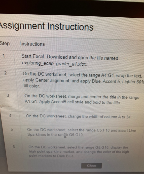
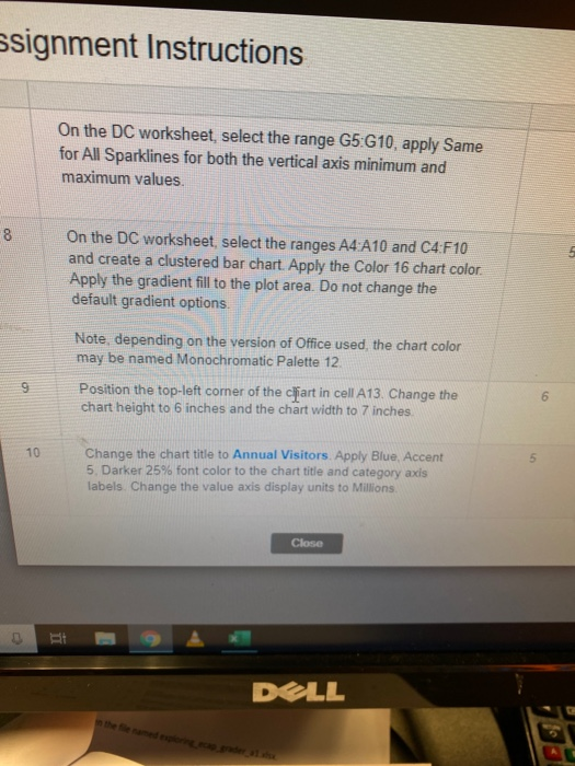
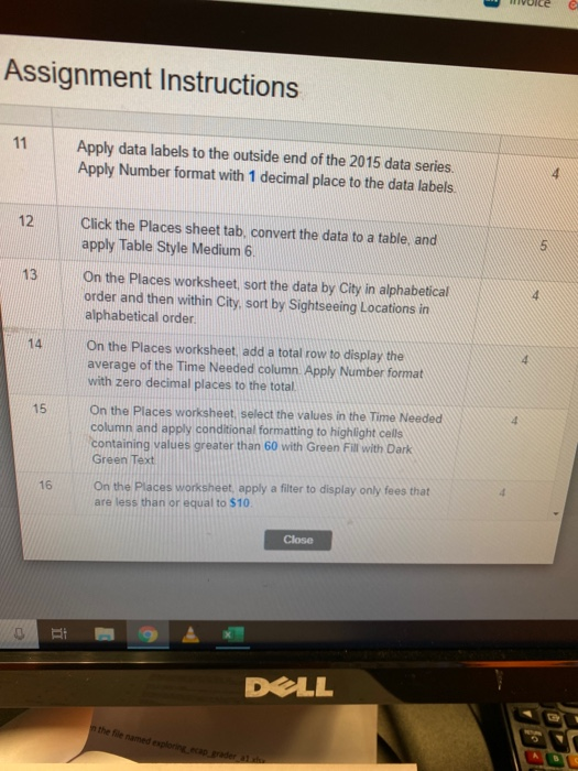
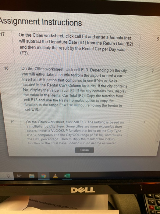
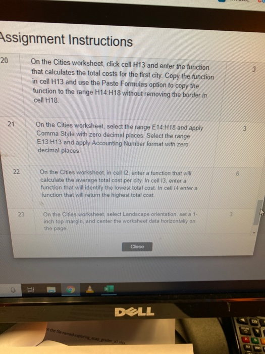
Assignment Instructions Step Instructions Start Excel. Download and open the file named exploring_ecap_grader_a1.xlsx On the DC worksheet, select the range A4:G4, wrap the text, apply Center alignment, and apply Blue, Accent 5. Lighter 60% fill color On the DC worksheet, merge and center the title in the range A1:G1. Apply Accents cell style and bold to the title. On the DC worksheet, change the width of column A to 34 On the DC worksheet, select the range C5:F10 and insert Line Sparklines in the range G5 G10. On the DC worksheet, select the range G5 G10 display the high point sparkline marker and change the color of the high point markers to Dark Blue Close ssignment Instructions On the DC worksheet, select the range G5:G10, apply Same for All Sparklines for both the vertical axis minimum and maximum values On the DC worksheet, select the ranges A4 A10 and C4:F10 and create a clustered bar chart. Apply the Color 16 chart color Apply the gradient fill to the plot area. Do not change the default gradient options. Note, depending on the version of Office used, the chart color may be named Monochromatic Palette 12. Position the top-left corner of the ciljart in cell A13. Change the chart height to 6 inches and the chart width to 7 inches Change the chart title to Annual Visitors. Apply Blue, Accent 5. Darker 25% font color to the chart title and category axis labels. Change the value axis display units to Millions Close DELL volce e Assignment Instructions 11 Apply data labels to the outside end of the 2015 data series. Apply Number format with 1 decimal place to the data labels 12 Click the Places sheet tab, convert the data to a table, and apply Table Style Medium 6. On the Places worksheet, sort the data by City in alphabetical order and then within City, sort by Sightseeing Locations in alphabetical order. On the Places worksheet, add a total row to display the average of the Time Needed column. Apply Number format with zero decimal places to the total On the Places worksheet, select the values in the Time Needed column and apply conditional formatting to highlight cells containing values greater than 60 with Green Fill with Dark Green Text 16 On the places worksheet, apply a filter to display only fees that are less than or equal to $10. Close DELL Assignment Instructions 17 On the Cities worksheet, click cell F4 and enter a formula that will subtract the Departure Date (B1) from the Return Date (B2) and then multiply the result by the Rental Car per Day value (F3). 18 On the Cities worksheet, click cell E13. Depending on the city, you will either take a shuttle to/from the airport or rent a car. Insert an IF function that compares to see if Yes or No is located in the Rental Car? Column for a city. If the city contains No, display the value in cell F2 If the city contains Yes, display the value in the Rental Car Total (F4). Copy the function from cell E13 and use the Paste Formulas option to copy the function to the range E14 E18 without removing the border in cell E18 19 On the Cities worksheet, click cell F13. The lodging is based on a multiplier by City Type. Some cities are more expensive than others Insert a VLOOKUP function that looks up the City Type (B13), compares it to the City/COL range (A7:B10), and returns the COL percentage Then multiply the result of the lookup function hy the Total Rasa lodnina (R51 to at the Astimated Close DELL the file medi e r Assignment Instructions 20 On the Cities worksheet, click cell H13 and enter the function that calculates the total costs for the first city. Copy the function in cell H13 and use the Paste Formulas option to copy the function to the range H14:H18 without removing the border in cell H18 W21 On the Cities worksheet, select the range E14 H18 and apply Comma Style with zero decimal places Select the range E13.H13 and apply Accounting Number format with zero decimal places On the Cities worksheet in cell 12. enter a function that will calculate the average total cost per city. In cell 13. enter a function that will identify the lowest total cost In cell 14 enter a function that will return the highest total cost. 23 On the Cities worksheet, select Landscape orientation set a 1- inch top margin and center the worksheet data horizontally on the page Close DOLL Assignment Instructions Step Instructions Start Excel. Download and open the file named exploring_ecap_grader_a1.xlsx On the DC worksheet, select the range A4:G4, wrap the text, apply Center alignment, and apply Blue, Accent 5. Lighter 60% fill color On the DC worksheet, merge and center the title in the range A1:G1. Apply Accents cell style and bold to the title. On the DC worksheet, change the width of column A to 34 On the DC worksheet, select the range C5:F10 and insert Line Sparklines in the range G5 G10. On the DC worksheet, select the range G5 G10 display the high point sparkline marker and change the color of the high point markers to Dark Blue Close ssignment Instructions On the DC worksheet, select the range G5:G10, apply Same for All Sparklines for both the vertical axis minimum and maximum values On the DC worksheet, select the ranges A4 A10 and C4:F10 and create a clustered bar chart. Apply the Color 16 chart color Apply the gradient fill to the plot area. Do not change the default gradient options. Note, depending on the version of Office used, the chart color may be named Monochromatic Palette 12. Position the top-left corner of the ciljart in cell A13. Change the chart height to 6 inches and the chart width to 7 inches Change the chart title to Annual Visitors. Apply Blue, Accent 5. Darker 25% font color to the chart title and category axis labels. Change the value axis display units to Millions Close DELL volce e Assignment Instructions 11 Apply data labels to the outside end of the 2015 data series. Apply Number format with 1 decimal place to the data labels 12 Click the Places sheet tab, convert the data to a table, and apply Table Style Medium 6. On the Places worksheet, sort the data by City in alphabetical order and then within City, sort by Sightseeing Locations in alphabetical order. On the Places worksheet, add a total row to display the average of the Time Needed column. Apply Number format with zero decimal places to the total On the Places worksheet, select the values in the Time Needed column and apply conditional formatting to highlight cells containing values greater than 60 with Green Fill with Dark Green Text 16 On the places worksheet, apply a filter to display only fees that are less than or equal to $10. Close DELL Assignment Instructions 17 On the Cities worksheet, click cell F4 and enter a formula that will subtract the Departure Date (B1) from the Return Date (B2) and then multiply the result by the Rental Car per Day value (F3). 18 On the Cities worksheet, click cell E13. Depending on the city, you will either take a shuttle to/from the airport or rent a car. Insert an IF function that compares to see if Yes or No is located in the Rental Car? Column for a city. If the city contains No, display the value in cell F2 If the city contains Yes, display the value in the Rental Car Total (F4). Copy the function from cell E13 and use the Paste Formulas option to copy the function to the range E14 E18 without removing the border in cell E18 19 On the Cities worksheet, click cell F13. The lodging is based on a multiplier by City Type. Some cities are more expensive than others Insert a VLOOKUP function that looks up the City Type (B13), compares it to the City/COL range (A7:B10), and returns the COL percentage Then multiply the result of the lookup function hy the Total Rasa lodnina (R51 to at the Astimated Close DELL the file medi e r Assignment Instructions 20 On the Cities worksheet, click cell H13 and enter the function that calculates the total costs for the first city. Copy the function in cell H13 and use the Paste Formulas option to copy the function to the range H14:H18 without removing the border in cell H18 W21 On the Cities worksheet, select the range E14 H18 and apply Comma Style with zero decimal places Select the range E13.H13 and apply Accounting Number format with zero decimal places On the Cities worksheet in cell 12. enter a function that will calculate the average total cost per city. In cell 13. enter a function that will identify the lowest total cost In cell 14 enter a function that will return the highest total cost. 23 On the Cities worksheet, select Landscape orientation set a 1- inch top margin and center the worksheet data horizontally on the page Close DOLL