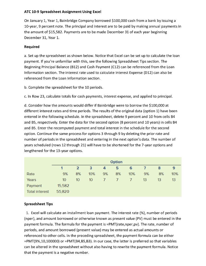
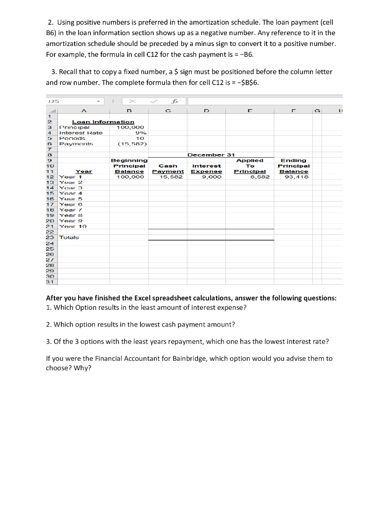
ATC 10-9 Spreadsheet Assignment Using Excel On January 1, Year 1, Bainbridge Company borrowed $100,000 cash from a bank by issuing a 10-year, 9 percent note. The principal and interest are to be paid by making annual payments in the amount of $15,582. Payments are to be made December 31 of each year beginning December 31, Year 1. Required a. Set up the spreadsheet as shown below. Notice that Excel can be set up to calculate the loan payment. If you're unfamiliar with this, see the following Spreadsheet Tips section. The Beginning Principal Balance (B12) and Cash Payment (C12) can be referenced from the Loan Information section. The interest rate used to calculate Interest Expense (012) can also be referenced from the Loan Information section. b. Complete the spreadsheet for the 10 periods. C. In Row 23, calculate totals for cash payments, interest expense, and applied to principal. d. Consider how the amounts would differ if Bainbridge were to borrow the $100,000 at different interest rates and time periods. The results of the original data (option 1) have been entered in the following schedule. In the spreadsheet, delete 9 percent and 10 from cells B4 and B5, respectively. Enter the data for the second option (8 percent and 10 years) in cells B4 and B5. Enter the recomputed payment and total interest in the schedule for the second option. Continue the same process for options 3 through 9 by deleting the prior rate and number of periods in the spreadsheet and entering in the next option's data. The number of years scheduled (rows 12 through 21) will have to be shortened for the 7-year options and lengthened for the 13-year options. 1 9% 10 15,582 55,820 2 8% 10 3 10% 10 4 9% 7 Option 5 8% 7 6 10% 7 7 9% 13 8 8% 13 9 10% 13 Rate Years Payment Total interest Spreadsheet Tips 1. Excel will calculate an installment loan payment. The interest rate %), number of periods (nper), and amount borrowed or otherwise known as present value (PV) must be entered in the payment formula. The formula for the payment is EPMT(rate,nper,pv). The rate, number of periods, and amount borrowed (present value) may be entered as actual amounts or referenced to other cells. In the preceding spreadsheet, the payment formula can be either =PMT(9%, 10,100000) or EPMT(B4,B5,B3). In our case, the latter is preferred so that variables can be altered in the spreadsheet without also having to rewrite the payment formula. Notice that the payment is a negative number. 2. Using positive numbers is preferred in the amortization schedule. The loan payment (cell B6) in the loan information section shows up as a negative number. Any reference to it in the amortization schedule should be preceded by a minus sign to convert it to a positive number. For example, the formula in cell C12 for the cash payment is =-B6. 3. Recall that to copy a fixed number, a $ sign must be positioned before the column letter and row number. The complete formula then for cell C12 is = -$B$6. 125 - LOAN Information Principal 100.000 Interest Rate 996 5 Periods 10 Payments (15,582) NOOPINION December 31 Beginning Applied Principal Caph Interest To Balance Payment Expense Principal 100,000 15,582 9,000 6,582 Ending Principal Balance 93,418 Year Year 1 Year 2 Year 3 Year 4 Your 5 Year 6 Year Year 8 Year 9 Year 10 Totals 12 31 After you have finished the Excel spreadsheet calculations, answer the following questions: 1. Which Option results in the least amount of interest expense? 2. Which option results in the lowest cash payment amount? 3. Of the 3 options with the least years repayment, which one has the lowest interest rate? If you were the Financial Accountant for Bainbridge, which option would you advise them to choose? Why? ATC 10-9 Spreadsheet Assignment Using Excel On January 1, Year 1, Bainbridge Company borrowed $100,000 cash from a bank by issuing a 10-year, 9 percent note. The principal and interest are to be paid by making annual payments in the amount of $15,582. Payments are to be made December 31 of each year beginning December 31, Year 1. Required a. Set up the spreadsheet as shown below. Notice that Excel can be set up to calculate the loan payment. If you're unfamiliar with this, see the following Spreadsheet Tips section. The Beginning Principal Balance (B12) and Cash Payment (C12) can be referenced from the Loan Information section. The interest rate used to calculate Interest Expense (012) can also be referenced from the Loan Information section. b. Complete the spreadsheet for the 10 periods. C. In Row 23, calculate totals for cash payments, interest expense, and applied to principal. d. Consider how the amounts would differ if Bainbridge were to borrow the $100,000 at different interest rates and time periods. The results of the original data (option 1) have been entered in the following schedule. In the spreadsheet, delete 9 percent and 10 from cells B4 and B5, respectively. Enter the data for the second option (8 percent and 10 years) in cells B4 and B5. Enter the recomputed payment and total interest in the schedule for the second option. Continue the same process for options 3 through 9 by deleting the prior rate and number of periods in the spreadsheet and entering in the next option's data. The number of years scheduled (rows 12 through 21) will have to be shortened for the 7-year options and lengthened for the 13-year options. 1 9% 10 15,582 55,820 2 8% 10 3 10% 10 4 9% 7 Option 5 8% 7 6 10% 7 7 9% 13 8 8% 13 9 10% 13 Rate Years Payment Total interest Spreadsheet Tips 1. Excel will calculate an installment loan payment. The interest rate %), number of periods (nper), and amount borrowed or otherwise known as present value (PV) must be entered in the payment formula. The formula for the payment is EPMT(rate,nper,pv). The rate, number of periods, and amount borrowed (present value) may be entered as actual amounts or referenced to other cells. In the preceding spreadsheet, the payment formula can be either =PMT(9%, 10,100000) or EPMT(B4,B5,B3). In our case, the latter is preferred so that variables can be altered in the spreadsheet without also having to rewrite the payment formula. Notice that the payment is a negative number. 2. Using positive numbers is preferred in the amortization schedule. The loan payment (cell B6) in the loan information section shows up as a negative number. Any reference to it in the amortization schedule should be preceded by a minus sign to convert it to a positive number. For example, the formula in cell C12 for the cash payment is =-B6. 3. Recall that to copy a fixed number, a $ sign must be positioned before the column letter and row number. The complete formula then for cell C12 is = -$B$6. 125 - LOAN Information Principal 100.000 Interest Rate 996 5 Periods 10 Payments (15,582) NOOPINION December 31 Beginning Applied Principal Caph Interest To Balance Payment Expense Principal 100,000 15,582 9,000 6,582 Ending Principal Balance 93,418 Year Year 1 Year 2 Year 3 Year 4 Your 5 Year 6 Year Year 8 Year 9 Year 10 Totals 12 31 After you have finished the Excel spreadsheet calculations, answer the following questions: 1. Which Option results in the least amount of interest expense? 2. Which option results in the lowest cash payment amount? 3. Of the 3 options with the least years repayment, which one has the lowest interest rate? If you were the Financial Accountant for Bainbridge, which option would you advise them to choose? Why